Optimal robust control under uncertainty
Contents |
Object
The optimal control relies on a model of the physical phenomenon to predict its future state and uses this information to derive the control distribution to be applied. The objective in this work is to account for the uncertainty which affects the system and significantly decreases the control performance. This uncertainty may come from poorly known boundary conditions, material properties and model unknowns. While the deterministic control gives good performance for a specific operating point only, the robust control should provide reasonable performance on a whole range of parameters.
Description
The considered configuration is one of a circular cylinder in cross-flow. The system is assumed 2-D for simplicity but the method is readily applicable to a 3-D configuration. The goal here is to determine the time distribution of blowing or suction at the cylinder surface to achieve a minimal drag while limiting the control intensity  to a minimum. The system uncertainty comes from the poorly known Reynolds number
  of the flow and is characterized by a probability distribution function
  . This configuration is supposed to be representative of the flow around the wing of an airplane during the flight which Mach number, and thus the flow Reynolds number, is fluctuating within a certain range.
Results and prospects
Using recent techniques of uncertainty propagation (e.g. polynomial chaos), a stochastic numerical code was written which simulates the flow and allows to know the statistical properties of all the variables of the problem and the drag Drag in particular. One has then to minimize the objective function  defined as
 where
where  ,
,  and
and  are constants to prescribe, weighting the contribution of the different terms of the functional,
  is the time horizon of the control and
  is a random event.
  is the optimal perturbation leading to the worst performances possible (
 -formulation of the control). The optimal control in the functional sense is determined by an adjoint method. Its temporal evolution is plotted in figure 1 (solid line). Comparing with the control distribution determined for the problem involving a deterministic (instead of random) Reynolds number
  (dashed line),
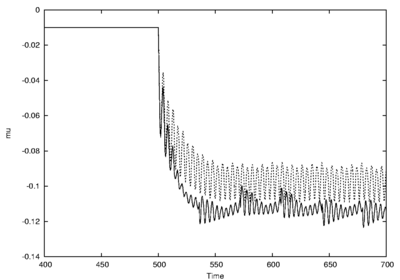
 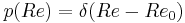 , it is clear that the robust control is less dependent on the vortex shedding phase. Figure 2 shows how the cylinder drag is affected by the control. The drag oscillation is strongly reduced while its mean value significantly decreases.
  (dashed line); robust control (solid line). The control is activated at (dashed line); robust control (solid line). The control is activated at  . . |
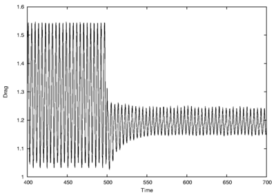 |
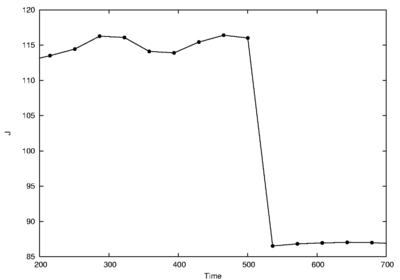
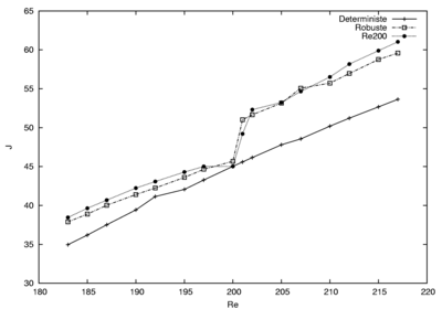
Figure 3 presents the time-evolution of the cost function. The control is seen to dramatically reduce the value of the objective function. On figure 4 the plot shows the functional evolution with the Reynolds number for the robust and the deterministic control together with the functional evolution for the control determined at . If the deterministic control gives, as expected, the best performance at the Reynolds number for which it was determined, its validity is very limited and its performance decays very fast when the determined control distribution is applied to a flow at a different Reynolds number. On the contrary, the robust control distribution, while less effective for a specific Reynolds number yields a more robust behavior in the sense that its performance less depends on the Reynolds number of the flow to which the control distribution is applied.
One of the next steps is to guarantee a minimal probability of achieving a performance lower than a certain prescribed limit.
 |
 |