Boundary conditions for natural convection around a heated wire

From 2007 Scientific Report

Jump to: navigation, search

M.-C. Duluc, S. Xin, F. Lusseyran and P. Le Quéré

1 Objectives
2 Experimental setup
3 Numerical simulations
4 Comparisons and discussion
5 References
6 Links

Objectives

The computation of the natural convection flow induced by a heated element placed in a very large environment remains a difficult task, owing to a lack of appropriate treatment to impose the far field boundary conditions. Two common practices can be found in the literature. Either one solves the equations in a very large domain, imposing in general no slip and isothermal conditions at the far field boundary. Previous investigations have shown that the computational domain has to be very large for the solution to converge, resulting in very large number of grid points and prohibitive computational costs. The alternative is to consider a computational domain of relatively small extension compared to the size of the source and the difficulty then lies in deriving appropriate boundary conditions. These boundary conditions should allow for a correct fluid entrainment on the inflow part and allow for fluid exit on the outflow, with the additional difficulty that the inflow and outflow parts are not known in advance and may furthermore change during the transient. In any case, checking the validity of different ways to impose these boundary conditions requires detailed experimental data. To this aim, a series of experiments were performed consisting of a stepwise heating of a small platinium wire and detailed measurements were made using PIV and temperature measurements.

Experimental setup

A thin platinum wire 100 $\mu \rm m$ in diameter (2R) and 5 cm in length is immersed in a large pool of demineralised water. In order to limit temperature variation of the bath, the container is inserted in a bigger cavity also filled up with demineralised water. The whole system is initially at room conditions. The water free surface is about 15 cm above the wire. Photographs of the experimental set-up are presented in Figure 1.

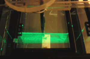
Figure 1: Top view of the experimental set-up. A vertical laser sheet, required for PIV measurements, is located perpendicularly to the horizontal wire

Velocity fields are measured by PIV techniques. A vertical laser light sheet is located perpendicularly to the horizontal wire and midway between the wire ends in order to avoid end effects. Seeding is achieved by polyacid particles of 20 µm in diameter and 1.03 in density. A CCD camera with a 8 bits resolution (768×484 pixels) is used. Each recording consists of a series of 600 pictures, the time delay between two neighboring frames being either 1/15 s or 1/30 s. The instantaneous 2D velocity field is obtained from a pair of neighboring frames by an original method based on optical flow algorithm [1]. The wire, heated by Joule effect, is connected to a power supply. The stepwise heating is performed using a relay of very short closing time (about 7 µs). The electrical circuit enables to realize heating steps of various magnitude and duration. Temperature measurements in the plume have also been carried out by using a K-type micro-thermocouple of 12.7 µm in diameter. Investigations have been conducted with three values of the applied heat flux: 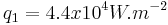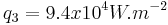$q_1=4.4x10^4 W.m^{-2}$ , $q_2=6.8x10^4 W.m^{-2}$ , $q_3=9.4x10^4 W.m^{-2}$ . The relevant Rayleigh numbers remain well under unity whatever the heat flux.

Numerical simulations

In the numerical approach, the fluid flow around the heated wire is assumed to be two-dimensional and obeys the Boussinesq approximation. The governing Navier-Stokes equations are expressed in polar coordinates [2]. The conditions imposed at the outer edge of the computational domain are the following :

$\frac {\partial T}{\partial r}= 0$		and		$\nu \left( \frac {\partial}{\partial r} + \frac{1}{r} \right) u = \frac{p}{\rho}$
				$\nu \left( \frac {\partial}{\partial r} + \frac{1}{r} \right) v =0$

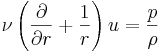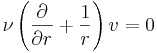Equations are discretized in time by a second-order scheme of finite difference type: for stability reasons the diffusion terms are treated implicitly while convective terms are treated explicitly. The spatial approximation makes use of basis functions made of tensor products of Chebyshev polynomials and Fourier series due to the periodicity in the azimuthal direction. In order to obtain adapted mesh distribution, a domain decomposition technique is used in radial direction. The domain $[R,R_0]$ is divided into several sub-domains and over each sub-domain a Chebyshev collocation method and a Fourier Galerkin method are used. Continuity of both functions and their first radial derivatives at the sub-domain interfaces is imposed by means of Schur complement. The velocity-pressure coupling is enforced by a standard projection method making use of time-splitting.

Comparisons and discussion

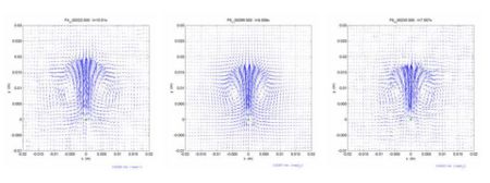
Figure 2 : Velocity fields measured by PIV at $tq^{1/2} = 21$ . The corresponding times are equal to respectively 10 s for $q_1$ (left), 8 s for $q_2$ (middle) and 7 s for $q_3$ (right). As can be seen, the flow structures are quite similar in geometry and spatial extension.

Numerical and experimental comparisons allowed validating previously established scaling laws of $t \sim q^{-1/2}\$ , $\delta r \sim q^{-1/4}\$ and $v \sim q^{1/4}\$ [3]. Although these laws were derived from a scaling analysis of the early onset of convective motion, the present study shows that these laws are still valid at longer times.

As an illustration are presented in Fig. 2, the velocity fields measured for the three heat fluxes for the same dimensionless time $tq^{1/2} = 21$ . The corresponding times are equal to respectively 10 s for $q_1$ (left), 8 s for $q_2$ (middle) and 7 s for $q_3$ (right). The flow structures are quite similar in geometry and extension. Similar results have been obtained for various values of the dimensionless time.

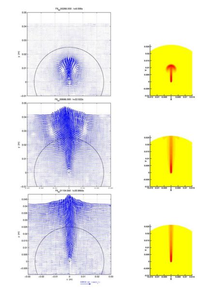
Figure 3 : A three-stage scenario of transient external natural convection.

Quantitative comparisons have also been performed [4]. The revealed that form a computational standpoint three different stages must be distinguished. These are illustrated in Fig. 3: Velocity fields measured by PIV are displayed on the left and temperature fields obtained by numerical simulation on the right. The boundary of computational domain ( $R_0 = 525R$ ) is shown as the black arc on the measured velocity fields. During the first stage (top), the induced flow and temperature fields are mainly inside of the computation demain. During the second one (middle), the two vortices and temperature front approach, cross and leave the outer boundary. On the third stage (bottom), the two vortices and temperature front are far away from the computional domain.

In the first stage the initial vortices are integrally included inside the computational domain. In this case, a good agreement is achieved between experiments and numerical simulations in the entire computational domain.

The second stage starts when the initial vortices and the front of the thermal plume reach up to the edge of the computational domain and finishes when they have totally passed through the outer boundary. These values depend on the numerical parameters. During this second stage, a good agreement is achieved between experiments and numerical simulations away from the outflow boundary.

In the ultimate stage, the initial vortices have left the computational domain and a quasi-steady laminar flow establishes around the wire. A good agreement between experimental and numerical results is achieved in the plume main stream as well as in the limited circle whose radius equals one third of the computational domain radius.

Figure 4 : Comparison of the vortex centers location

Experiments have shown that the initial vortices' centers follow a linear path which is almost independent of the heating rate (Fig. 4). An analytical law of $y = \mp 2.5 \times (x \pm 0.001)\$ is proposed for the linear path. This yields the vertical position of -0.0025 m for the virtual source. The numerical prediction for the trajectory of the vortex center is only valid for Stage 1.

References

[1] G.M. Quénot, J. Pakleza, and T.A. Kowalewski. Particle image velocimetry with optical flow. Exp. Fluids, 25:177–189, 1998.

[2] S. Xin, M.-C. Duluc, F. Lusseyran, and P. Le Quéré. Numerical simulations of natural convection around a line-source. Int. J. Num. Meth. Heat & Fluid Flow, 14(7):828–848, 2004.

[3] M.-C. Duluc, S. Xin, and P. Le Quéré. Transient natural convection and conjugate transients around a line heat source. Int. J. Heat Mass Trans., 46:341–354, 2003.

[4] M.-C. Duluc, S. Xin, F. Lusseyran, and P. Le Quéré. Numerical and experimental investigation of laminar free convection around a line-source: long time scalings and assessment of numerical approach. submitted to Int. J. Heat Fluid Flow.

Links

CORO