An hybrid spectral-finite element method for the 3D MagnetoHydroDynamics equations in heterogeneous domains
C Nore, R Laguerre and A Ribeiro in collaboration with J.-L. Guermond (Texas A&M University, USA) and J. Léorat (*)
(*) Laboratoire Univers et Théories (LUTh) Observatoire de Paris, CNRS, Université Paris Diderot 5 Place Jules Janssen - 92195 Meudon Cedex
Contents |
Object
The purpose of this paper is to demonstrate the ability of a
new Spectral-Finite Element Method (SFEMHD) algorithm
to deal with situations described by the MagnetoHydroDynamics (MHD)
equations in the presence
of conducting and nonconducting regions. In various axisymmetric domains,
we have considered ohmic diffusion in conductors or
induction in solid rotors submitted to a uniform and constant magnetic field.
Comparisons have shown good agreement with
analytical or previously published numerical solutions in two and
three dimension configurations.
We also simulate the kinematic dynamo action in different geometries
and currently we are investigating the nonlinear version of the code.
More specifically, we present here two cases of
kinematic dynamos where the velocity field is imposed and the magnetic field
can grow or decay depending on the value of the order parameter, namely the
magnetic Reynolds number  .
.
Overview of the numerical method
In this section we give a brief overview of the numerical method which is used. The problem is modeled by the MHD equations in the eddy current approximation with no retroaction of the magnetic field on the velocity field (kinematic dynamo approximation):
with relevant boundary and initial data,
where  is the magnetic field,
  the electric field,
 an imposed velocity field,
 the electric conductivity and
  the magnetic permeability.
This system is solved in a heterogeneous domain composed
of conducting regions of different
conductivities (
the magnetic permeability.
This system is solved in a heterogeneous domain composed
of conducting regions of different
conductivities (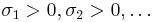 ) and an insulating region (vacuum,
  ).
Since the magnetic field is curl free in vacuum,
it can be expressed as the gradient of a scalar potential
).
Since the magnetic field is curl free in vacuum,
it can be expressed as the gradient of a scalar potential  ,
as long as the insulating domain is simply connected.
can then be eliminated and the original system can be re-written
in term of and only (see reference [1]).
Enforcing continuity of and
,
as long as the insulating domain is simply connected.
can then be eliminated and the original system can be re-written
in term of and only (see reference [1]).
Enforcing continuity of and  across
interfaces is a significant numerical difficulty.
In our finite element approximation,
continuity is not enforced in the function spaces but is rather weakly imposed using
an Interior Penalty Galerkin method (IPG) together with Lagrange elements.
This method has been shown to be stable and convergent in [1].
across
interfaces is a significant numerical difficulty.
In our finite element approximation,
continuity is not enforced in the function spaces but is rather weakly imposed using
an Interior Penalty Galerkin method (IPG) together with Lagrange elements.
This method has been shown to be stable and convergent in [1].
Since the geometry is axisymmetric,
the equations are written
in cylindrical coordinates and the approximate solution
is expanded in Fourier series in the azimuthal direction and
nodal Lagrange finite elements in the meridian plane.
The time is discretized by means of a semi-implicit
Backward Finite Difference method of second order
(BDF2). If the boundary of the computational domain is the vacuum boundary, we can impose
Robin, Neumann, or Dirichlet boundary conditions on .
Results
We focus here on the kinematic dynamo problem, in which the velocity field is imposed
and the magnetic field is free to evolve. Note that
 is a solution of the MHD equations which becomes
unstable above criticality. The order parameter
is a solution of the MHD equations which becomes
unstable above criticality. The order parameter
 is the magnetic Reynolds number based
on the characteristic velocity
is the magnetic Reynolds number based
on the characteristic velocity  and length
  . It compares
the production term to the dissipative term.
. It compares
the production term to the dissipative term.
Dynamo in the Perm torus
The configuration we model is inspired from the so-called
Perm device [2].
This experiment aims at generating the dynamo effect in a strongly
time-dependent helical flow created in a toroidal channel
after impulsively stopping the fast rotating container.
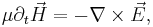
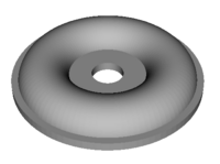
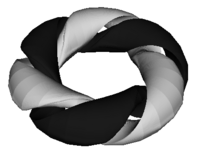
We consider a torus which is represented on figure 1.
The reference length scale
is chosen so that the nondimensional mean radius of the torus
(the distance between the  -axis and the center
of the cross section) is
-axis and the center
of the cross section) is  .
The nondimensional radius of the circular cross section is
.
The nondimensional radius of the circular cross section is  .
The inner part of the torus,
.
The inner part of the torus,  , is occupied by
conducting fluid of conductivity
, is occupied by
conducting fluid of conductivity  and is referred to as the fluid channel.
The outer part of the torus,
and is referred to as the fluid channel.
The outer part of the torus,  is occupied by
conducting solid of conductivity
is occupied by
conducting solid of conductivity  . In order to be closer to the real experimental geometry,
the conducting domain includes flat equatorial protuberances (see figure 1).
The numerical domain has the following discretization characteristics:
the conducting domain is discretized using a quasi-uniform grid
of meshsize
. In order to be closer to the real experimental geometry,
the conducting domain includes flat equatorial protuberances (see figure 1).
The numerical domain has the following discretization characteristics:
the conducting domain is discretized using a quasi-uniform grid
of meshsize  and is embedded in a spherical insulating domain of radius 10.
The flow velocity is helical with a uniform azimuthal component that we
henceforth denote by  . The reference velocity
 is chosen to be
 so that the magnetic Reynolds number can be rewritten as
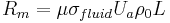 .
The non-dimensional helical flow in the fluid channel is then defined in cylindrical
coordinates by
.
The non-dimensional helical flow in the fluid channel is then defined in cylindrical
coordinates by
 where
where  is a constant hereafter referred to
as the poloidal to toroidal velocity ratio.
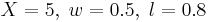
We choose
is a constant hereafter referred to
as the poloidal to toroidal velocity ratio.
We choose  .
.
Since the flow is axisymmetric, the magnetic azimuthal
modes evolve independently;
therefore, the initial magnetic field
in the conductor is set
to contain all the azimuthal modes that we want to test.
After thorough investigations, we have found that
 is the critical mode corresponding to the lowest
critical magnetic Reynolds number.
More precisely we have determined
is the critical mode corresponding to the lowest
critical magnetic Reynolds number.
More precisely we have determined  .
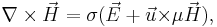
We show in figure 2 (a-b) the
.
We show in figure 2 (a-b) the  -component
of the unstable mode at
-component
of the unstable mode at  .
Observe that the support of this unstable eigenmode is localized close
to
.
Observe that the support of this unstable eigenmode is localized close
to  , in the region of maximum shear.
This eigenmode has a double helix shape and has the same helicity sign as
that of the velocity field. It is rotating in a retrograde sense
with a period of
, in the region of maximum shear.
This eigenmode has a double helix shape and has the same helicity sign as
that of the velocity field. It is rotating in a retrograde sense
with a period of  (see figure 2 a-b).
Our computations are the only ones performed in a torus.
For more details, see reference [1].
(see figure 2 a-b).
Our computations are the only ones performed in a torus.
For more details, see reference [1].
 |
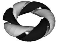  at at  : iso-surfaces of the : iso-surfaces of the  component of the mode; component of the mode;  of the minimum value in black and of the minimum value in black and  of the maximum value in white of the maximum value in white |
  |
Dynamo in the rotating MND flow
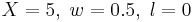
We now examine a rotating flow in a cylindrical cavity of
unit height-to-diameter aspect ratio.
The conducting domain, composed of a finite cylinder (fluid)
and an additional external layer (vessel),
is discretized using a quasi-uniform grid
of meshsize  .
The conducting region is embedded
in a spherical insulating domain of radius 10.
The fluid flow is modeled by the following
so-called MND velocity field [3],
used as a convenient simplified model of the actual VKS (von Kármán Sodium) flow, expressed
in cylindrical coordinates
.
The conducting region is embedded
in a spherical insulating domain of radius 10.
The fluid flow is modeled by the following
so-called MND velocity field [3],
used as a convenient simplified model of the actual VKS (von Kármán Sodium) flow, expressed
in cylindrical coordinates  :
:
for  and
and  :
:

The parameter  is the toroidal to poloidal flow ratio. We use
 which yields near optimal dynamo action,
as shown in [3]. Since the flow is axisymmetric, the magnetic azimuthal
modes evolve independently; as a result,
we restrict ourselves to the azimuthal mode 1 which
is known to be the most unstable.
Hereafter, we use the following definition
of the magnetic Reynolds number:
which yields near optimal dynamo action,
as shown in [3]. Since the flow is axisymmetric, the magnetic azimuthal
modes evolve independently; as a result,
we restrict ourselves to the azimuthal mode 1 which
is known to be the most unstable.
Hereafter, we use the following definition
of the magnetic Reynolds number:  ,
where
,
where  is the radius of the
inner cylinder and
is the radius of the
inner cylinder and  the maximum of the velocity.
The vessel containing the fluid is a hollow cylinder (see
figure 4 a).
The nondimensional thickness of the side wall is denoted by
the maximum of the velocity.
The vessel containing the fluid is a hollow cylinder (see
figure 4 a).
The nondimensional thickness of the side wall is denoted by  and that of the top and bottom lids is denoted by
  .
The conductivity ratio
.
The conductivity ratio
 is
denoted by
is
denoted by  .
.
Inspired by a previous study [5], we study the influence of conducting annuli and top and bottom lids, .
We first consider a vessel having the shape of a cylindrical annulus, i.e.
the thickness of the lids is first assumed to be infinitely thin ( ),
(see figure 4 b, case S).
Figure 3(a) shows
),
(see figure 4 b, case S).
Figure 3(a) shows
 as a function of for
  and
and  .
We observe that
.
We observe that  decreases quasi-exponentially with respect to
at with the typical lengthscale
decreases quasi-exponentially with respect to
at with the typical lengthscale  ,
thus confirming results from [4],
then reaches an asymptote for large .
,
thus confirming results from [4],
then reaches an asymptote for large .
We now set the thickness of the annulus to  , and
we analyze the effect of top and bottom lids of thickness .
This case has been studied in [5]
with no conductivity jump, i.e. ,
the main result being that dramatically increases with respect to .
We display in figure 3(b)
, and
we analyze the effect of top and bottom lids of thickness .
This case has been studied in [5]
with no conductivity jump, i.e. ,
the main result being that dramatically increases with respect to .
We display in figure 3(b)
 as a
function of for and .
We observe that increases with and
that this effect is again amplified by the conductivity jump, the
variation being the largest in the range
as a
function of for and .
We observe that increases with and
that this effect is again amplified by the conductivity jump, the
variation being the largest in the range  .
.
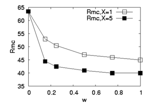 as a function of conducting annulus width for and as a function of conducting annulus width for and |
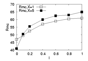 as a function of conducting top and bottom lid height for and with a fixed wall thickness as a function of conducting top and bottom lid height for and with a fixed wall thickness |
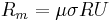
To better comment on the behavior of with respect to and ,
we now compare the spatial distribution
of dissipation and currents in three typical cases:
(i) case N: No envelope;
(ii) case S (Side): an annulus of thickness with and no lids ;
(iii) case SL (Side-Lids): an annulus of thickness
and two lids of thickness  with .
The results are reported in figure 4 (a-c).
with .
The results are reported in figure 4 (a-c).
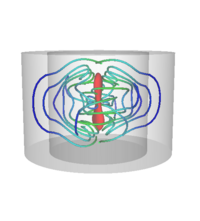
For the cases N and S, most of the dissipation is concentrated in the fluid, close to the cylinder axis, whereas in the SL case, new dissipation patterns occur within the lids. The figure shows some characteristic lines of the current vector field. The spatial distribution of the lines close to the axis is pretty similar in the three cases, but it significantly differs in regions close to the envelope. Going from the case N to the case S, the currents formerly constrained in the flow volume are deformed and expand to fill the annulus on large scales, suggesting that the dissipation decreases as indeed observed. Going from the case S to the case SL, additional current loops at small scales appear within the top and bottom lids leading to more Ohmic dissipation. For more details, see reference [6].
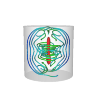  of the total dissipation and current lines for of the total dissipation and current lines for  and and  |
  and and 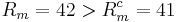 |
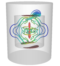  and and 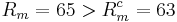 |
Discussion and conclusion
We have shown the ability of our SFEMANS (Spectral Finite Element Maxwell And Navier-Stokes) code to simulate kinematic dynamo action in various geometries with different physical properties. Our results confirm that the impact of an envelope is crucial for the design of experimental fluid dynamos and this effect is enhanced by the difference of vessel and fluid conductivities. In the near future, we plan to optimize the geometry of the envelope of the VKS (von Kármán Sodium) set-up by using the experimental mean flow [4] and the actual sizes and conductivities of the materials that are used (sodium, copper, stainless steel). We are also studying the nonlinear dynamo action in a Taylor-Couette flow between two finite cylinders.
References
[1] J.-L. Guermond, R. Laguerre, J. Léorat and C. Nore, A Discontinuous Galerkin Method for the MHD equations in heterogeneous domains, J. Comp. Physics, 221, 349-369 (2007).
[2] W. Dobler, P. Frick and R. Stepanov, Screw dynamo in a time-dependent pipe flow, Phys. Rev. E, 67, 056309 (2003).
[3] L. Marié, C. Normand and F. Daviaud, Galerkin analysis of kinematic dynamos in the von Kármán geometry, Phys. Fluids, 18, 017102 (2006).
[4] F. Ravelet, A. Chiffaudel, F. Daviaud, J. Léorat, Towards an experimental von Kármán dynamo: numerical studies for an optimized design, Phys. Fluids, 17, 117104 (2005).
[5] F. Stefani, M. Xu, G. Gerbeth, F. Ravelet, A. Chiffaudel, F. Daviaud and J. Léorat, Ambivalent effects of added layers on steady kinematic dynamos in cylindrical geometry: application to the VKS experiment, Eur. J. Fluid Mech./B, 25, 894–908 (2006).
[6] R. Laguerre, C. Nore, J. Léorat and J.-L. Guermond, Induction effects of conductivity jumps in the envelope of a kinematic dynamo flow, C. R. Mécanique, 349-369 (2006).