Natural convection between infinite concentric cylinders
M. Prud'homme and P. Le Quéré
Contents |
Introduction
Many configurations of industrial interest are cylindrical containers isolated from their surroundings by an annular space filled with a low conductivity fluid such as air. The fluid in this annular space is submitted to a horizontal temperature difference resulting in a global motion whose net vertical mass flux is zero if the annular space is sealed at both ends. In many cases the container is set in an environment which is vertically thermally stratified. If the annular space is thin compared to its height one can assume that the flow takes place in an infinite annular slot whose wall temperatures increase linearly with height in such a way that at any elevation the temperature difference across the walls is constant. In the next section we will determine the base flow structure and the corresponding Nusselt number. One also wants to determine wether the base flow is stable, to determine the nature of the bifurcation, and to investigate the properties of the fully non-linear flows resulting from the instabilities.
Base flow
Consider the space between two vertical concentric cylinders of
inner and outer radius  and
and  . We assume that the wall
temperature of the innner cylinder is
. We assume that the wall
temperature of the innner cylinder is  and than that of the outer cylinder reads
  , where
  is a reference
temperature,
is a reference
temperature,  is the constant temperature difference
across the slot and
is the constant temperature difference
across the slot and  the constant vertical temperature
gradient. The slot is filled with a fluid of thermal diffusivity
the constant vertical temperature
gradient. The slot is filled with a fluid of thermal diffusivity
 and of kinematic diffusivity
  . We assume that the
fluid follows the Boussinesq approximation, ie
. We assume that the
fluid follows the Boussinesq approximation, ie  where
where  .
Looking for a parallel solution such as
.
Looking for a parallel solution such as 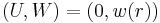 the
governing equations reduce to :
the
governing equations reduce to :
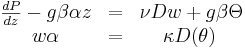
where 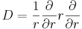 and
and
 . The left and right members of the first
equation are functions of
. The left and right members of the first
equation are functions of  and
and  respectively and thus equal to
a constant which can be written
respectively and thus equal to
a constant which can be written  , resulting in
the system :
, resulting in
the system :

Upon introducing  as reference length and
as reference temperature difference, the elimination of
as reference length and
as reference temperature difference, the elimination of
 between the two equations shows that $w$ satisfies the
fourth order differential equation :
between the two equations shows that $w$ satisfies the
fourth order differential equation :
 where
where  , and
, and  . Thus
  expresses as
 where
where  are Bessel functions and
  modified Bessel functions
of the first and second kind respectively with
modified Bessel functions
of the first and second kind respectively with  , and
, and  such as
 .
As
.
As  , it follows that
 Integrating this equation, making use of algebraic properties of Bessel
functions \cite{abram}
and imposing that the two walls are no-slip and iso-flowrates boundaries shows
that the 4 coefficients satisfy the following linear system
Integrating this equation, making use of algebraic properties of Bessel
functions \cite{abram}
and imposing that the two walls are no-slip and iso-flowrates boundaries shows
that the 4 coefficients satisfy the following linear system
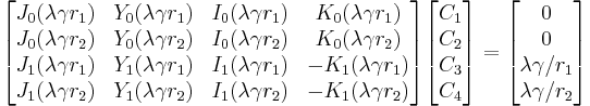
Due to the asymptotic behavior of the Bessel functions, this system becomes ill-conditioned when
the product  becomes large (values of 10 or so), that is when the solution is composed of two distinct boundary layers.
 |
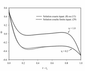 |
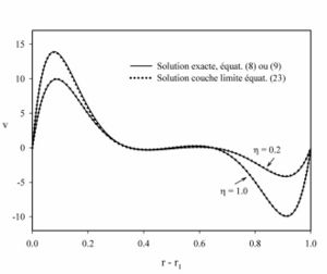
This situation provides an alternative way to determine the base flow, through a matched asymptotic expansion
of the inner and outer solutions. The procedure is described in Prud'homme and Le Quéré.
As expected the expansion converges quickly when the two boundary layers are indeed distinct, ie when the stream function achieves a constant value in the central core region. The figure above gives a comparison of the base flow solution obtained when both methods work equally well.
Both methods are thus complementary and provide access to the base flow solution for the entire range of governing parameters.
Linear instability
The stability of this base flow is first investigated in the
framework of the linear stability theory, ie under the assumption of
disturbances of infinitesimal amplitude expanded in normal modes.
Perturbations are written as 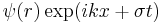 where
where  is the real wave umber and
 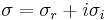 is the complex growth factor.
  corresponds to instability and
  is the wave speed.
The generalized eigenvalue problem is solved for fixed with the
help of the library. A secant method is used to determine the value
of
is the wave speed.
The generalized eigenvalue problem is solved for fixed with the
help of the library. A secant method is used to determine the value
of  for which
  . The linear stability was solved
for a wide range of and Prandtl number values.
. The linear stability was solved
for a wide range of and Prandtl number values.
 |
 |
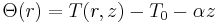
 ,
, 
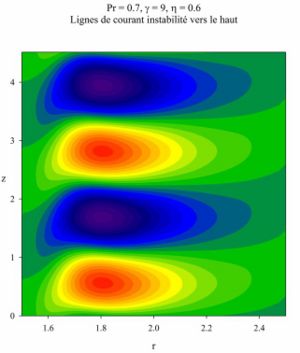
A sample result is presented in figure 2, corresponding to a flow of air in the case of strong curvature effects and a strong stratification. The figure shows that the instability mode is concentrated along the inner heated cylinder, and its phase velocity indicates that it is an upward moving wave.
Weakly nonlinear instability
Additional computations were performed in order to investigate the nature of the bifurcation. These calculations involve projection of the nonlinear on the adjoint of the most unstable eigenmode in order to compute the Landau coefficients. Details are given in Prud'homme and Le Quéré [1]. The results show that the Hopf bifurcation can be either subcritical or supercritical depending on the parameters.
References
[1] M. Prud'homme et P. Le Quéré, Stability of stratified natural convection in a tall vertical annular cavity, Physics of Fluids, (2007), 19, 094106.