The spectrum of glottal flow models
B. Doval, C d'Alessandro, with N. Henrich
Contents |
Object
Glottal source
Most of the speech features related to voice quality, vocal effort and prosodic variations can be associated with the voice source. In the source/filter model of speech production, this source is often described in terms of a glottal flow, and is modelled as a time-domain function called "glottal flow model", abbreviated GFM hereafter. Several GFMs have been proposed such as the well-known LF model (Liljencrants and Fant [5]), the KLGLOTT88 model (Klatt [6]), the Rosenberg's models [7] or the R++ model (Veldhuis [8]).
Voice quality
But in areas such as speech synthesis, voice quality analysis or speech processing, a frequency-domain approach appears to be desirable. Generally, voice quality is better described by spectral parameters, such as the spectral tilt, the relative amplitude of the first harmonics, the harmonic richness factor (Childers), the parabolic spectral parameter (Alku), etc. An interesting feature is the spectral peak that can be observed on the glottal flow derivative spectrum in the region of the first harmonics. This peak has been called "the glottal formant". The question is now: how to exhibit a link between voice quality and glottal source parameters? or in other words: What are the spectral correlates of the time-domain GFM parameters?
Spectral correlates of the time-domain GFM parameters
The main goal of this work is to give answers to this question. For that, it studies the position, variation and properties of the glottal formant in a unified framework, and gives explicit equations for relating time-domain glottal flow parameters to the glottal formant. This work has many outcomes :
- it defines the spectral behaviour of most common glottal flow models
- it gives the relationships between time-domain and spectral parameters
- it gives some hints for spectral estimation or modification of glottal flow parameters
This work is the closure of a study on glottal flow models ([2], [3], [4]) and has been published in Acta Acustica in 2006 (Doval et al. [1]).
Glottal flow models (GFMs)
Time-domain features and parameters
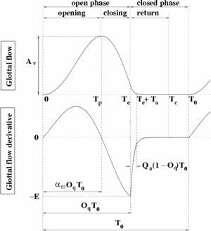
All the GFMs share some common time-domain features (cf. Figure 1) :
- the glottal flow is always positive or null
- the glottal flow and its derivative are quasi-periodic
- during a fundamental period, the glottal flow is bell-shaped: it increases, then decreases, then becomes null
- during a fundamental period, the glottal flow derivative is positive, then negative, then null.
- the glottal flow and its derivative are continuous and differentiable functions of time, except in some situations at the glottal closing instant (GCI).
GFMs are described in terms of phases:
- the opening phase: the glottal flow increases from baseline at time 0 to its maximum amplitude
 also called "amplitude of voicing" at time
  .
.
- the closing phase: the glottal flow decreases from to a point at time
 where the derivative reaches its negative extremum
  . is the glottal closing instant (GCI) and is called the "maximum excitation".
- the open phase: it is simply the set of the opening and closing phases, characterized by the open quotient
 . The ratio between the opening phase and the open phase is called "asymmetry coefficient" and noted
  .
.
- the closed phase:
- case "abrupt closure": in this case, there is a discontinuity in the glottal flow derivative which instantaneously reaches 0 after maximum excitation. The glottal flow is null between
 and
and  .
.
- case "smooth closure": the glottal flow derivative is continuous and exponentially returns to 0 at time
 . This phase is called "return phase" and the exponential time constant is noted
  . It can also be characterized by the relative parameter
 ![Q_a=T_a/[(1-O_q)T_0]](../upload/math/6/b/2/6b296f1ff035b16d25489c7f9269305d.png) which takes its value between 0 and 1.
which takes its value between 0 and 1.
- case "abrupt closure": in this case, there is a discontinuity in the glottal flow derivative which instantaneously reaches 0 after maximum excitation. The glottal flow is null between
The smooth closure case can be modelled in 2 different ways: either a time-domain decreasing exponential (leading to the return phase as described above) noted "return phase method" or a low-pass first (or second) order filter applied to the whole open phase noted "low-pass filter method".
Studied GFMs
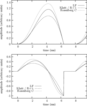 Figure 3
Among the GFMs proposed in the literature, we have studied the following ones:
- KLGLOTT88 model (Klatt): the glottal flow is modeled by a third order polynomial which is possibly smoothed using the low-pass filter method. There are 4 parameters: , ,
 and
and  which is the attenuation in dB of the low-pass filter at 3000 Hz. Notice that the asymmetry of the flow cannot be changed and is always:
  .
.
- R++ model (Veldhuis): the glottal flow is composed of a fourth order polynomial for the open phase followed by an exponential return phase. There are 5 parameters:
 (an amplitude coefficient), , , and . The glottal flow is computed so that it returns exactly to 0 at the end of the cycle.
- Rosenberg C (Rosenberg): the glottal flow is composed of 2 sinusoidal parts. The 4 parameters are: , , and
 . Noticed that the smooth closure case is not handled.
- LF model (Liljencrants and Fant): the glottal flow derivative is modelled by an exponentially increasing sinusoid followed by a decreasing exponential. There are 5 parameters:
 (the maximum excitation), , , , . The glottal flow is computed so that it returns exactly to 0 at the end of the cycle. For that, 2 implicit equations must be solved.
Figure 3 shows example of the 4 GFMs (top) and their derivatives (bottom) with abrupt closure and with a common set of parameters:  ,
,  , and
, and  . KLGLOTT88 and R++ models are identical for this parameter set. Note that differs between models when and the other parameters are fixed. However these differences are hardly audible.
Generic model
In order to be able to compare the different GFMs, a common set of 5 time-domain parameters have been chosen:
- , the maximum excitation
- , the fundamental period
- , the open quotient
- , the asymmetry coefficient
-
 , the return phase quotient
All the GFMs can be rewritten using this parameter set. Let us note  this set. Then we have shown that for the abrupt closure case, the glottal flow
  and its derivative can always be written on a single period as follows, whatever the model:

where  is a function of time
  which depends on only one parameter (). This function is called "the generic model" and concentrate all the uniqueness of a given model.
The amplitude of voicing and the total flow  can be expressed in function of the basic parameters, and the maximum of
  , noted
  , and the integral of , noted
  , respectively:

Spectral properties of GFMs
Low-pass filters
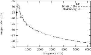
Since the early years of the source-filter theory of speech production, it is well known that the effect of the glottis in the spectral domain can be approximated by a low-pass system. When considering the GFM derivative spectrum, one can show that it behaves like a bandpass filter, and a spectral peak appears in low frequencies, which is called "glottal formant" hereafter. Figure 6 shows the spectra of the 4 GFM derivatives of Figure 3.
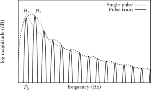
Figure 10 shows the spectrum of a pulse train rather than a single period for the LF model: harmonics are clearly visible and the glottal formant is situated around the first harmonics.
The analytic expression of the GFM spectrum and of the GFM derivative spectrum can deduced from the time domain equations by a Fourier transform:

This last equation shows that:
- has the effect of an overall gain
- allows the whole spectrum to stretch or shrink, the harmonic amplitudes and phases being unchanged
- has the same type of effect as but it stretches or shrinks only the spectral envelope, without changing the harmonic frequencies
- the effect of depends on the specific generic model used
Spectrum of the generic GFM and spectrum stylisation
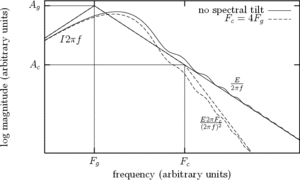
An analytic study of the asymptotes of the GFM derivative spectrum shows that the spectrum, represented in a log-log scale, can be stylized by 3 lines as can be seen in Figure 11:
- +6dB/oct:
- -6dB/oct:
 in the case of abrupt closure
- -12dB/oct:
 in the case of smooth closure
The crossing points of the asymptotes,  and
and  , completely define the stylized spectrum. Their values can be expressed in function of the time-domain parameters. In particular:

where  and
and  are the coordinates of the asymptote crossing point of
  .
.
An important conclusion is that the crossing point frequency  does not depend on , is proportionnal to
  , and
inversely proportionnal to . Its relation to
is the only dependence which is specific to each model.
, and
inversely proportionnal to . Its relation to
is the only dependence which is specific to each model.
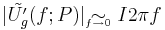
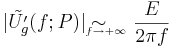
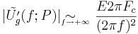
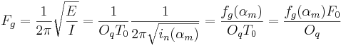
Glottal formant
Frequency and amplitude
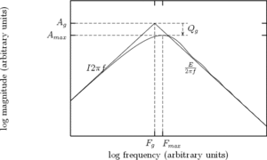
Most of the time, the GFM derivative spectrum follows quite regularly the asymptotes as shown Figure 11. The spectral maximum that appears in low frequency on the GFM derivative spectrum is an important feature for voice quality. It is called the "glottal formant", even if the term formant does not refer here to a resonance but only to a spectral maximum. A main goal of this study is to better understand the relationship between this glottal formant and the time-domain GFM parameters.
As can be seen Figure 8, the glottal formant takes place at a frequency slightly
higher than the asymptotes crossing point, and at an amplitude which can be
rather different. If we denote  and
and  the frequency and
amplitude of the glottal formant, then their relationship with the time-domain
parameters writes:
the frequency and
amplitude of the glottal formant, then their relationship with the time-domain
parameters writes:


Effects of and on the glottal formant
These equations shows that the dependence on , and are
proportional or inversely proportional relationships. Only parameter is model dependent.
It can be seen that:
- the glottal formant frequency hardly depends on
- it takes place roughly between the first and the 4th harmonic
- its relative amplitude depends mainly on
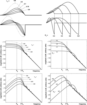
Figure 14 shows the influence of (right) and (left) on the GFM (middle) and the GFM derivative (bottom) spectra, E being fixed. Several points may be observed:
- the mid and high frequencies are not much modified by and variations
- mainly changes the glottal formant frequency
- mainly changes the glottal formant amplitude (or rather its bandwidth)
Spectral tilt
Return phase or low-pass filter
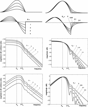
The spectral tilt denotes the behaviour of the GFM in mid to high frequencies. It has been shown to be related to the return phase in the case of smooth closure of the vocal cords (cf. Figure 1). From a modelling point of view, two methods can be applied: either a time-domain decreasing exponential (leading to the return phase as described above) noted "return phase method" or a low-pass first (or second) order filter applied to the whole open phase noted "low-pass filter method". For example, R++ and LF are using the "return phase method" while KLGLOTT88 is using the low-pass filter method.
The spectral tilt parameter is (cf. Figure 1). It has been shown that its main effect is to introduce an additional spectral -6dB/oct slope above the cut-off frequency  (cf. Figure 11). Figure 13 (right) illustrates the effect of .
The main effect of the spectral tilt corresponds to loud/soft voices: when
is low (or null), the spectral tilt is low, corresponding to a high (or
infinite) cut-off frequency, and the voice is loud ; when is high (near
1), the spectral tilt is high, corresponding to a low cut-off frequency, and
the voice is soft.
Applications
NAQ
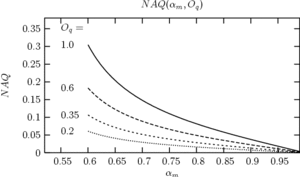
The voice quality modification due to the asymmetry coefficient
(or equivalently the speed quotient) is rarely described
in the literature. The time-domain parameter NAQ proposed by Alku [9] tries to
parametrize the glottal closing phase. It is defined by the
-normalized ratio between and .
From the above equation, it can be seen that NAQ is directly
related to and by:
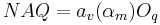 . Figure 12 shows this relationship for the
LF model. The equation shows that NAQ is proportional to and
decreases with and explain why this parameter is
considered to capture the relative degree of tenseness/laxness.
. Figure 12 shows this relationship for the
LF model. The equation shows that NAQ is proportional to and
decreases with and explain why this parameter is
considered to capture the relative degree of tenseness/laxness.
H1-H2
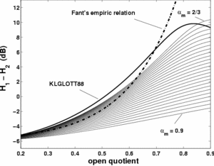
Another often used parameter is the difference between the 2 first harmonic
amplitudes  (Hanson [10]). It has been considered to be
strongly correlated to . Our development shows that its
dependence on is clear, but that it depends also on
, as shown in the following equation:
(Hanson [10]). It has been considered to be
strongly correlated to . Our development shows that its
dependence on is clear, but that it depends also on
, as shown in the following equation:

The precise dependence on is shown in Figure 18 for the
LF model. On the same Figure is plotted the curve obtained for the Klatt model
(which asymetry parameter is fixed at  ) and the Fant's empiric
relation between and .
) and the Fant's empiric
relation between and .
The main result is that a given value of does not
correspond to an unique value of but to an
interval as a function of .
References
[1] B. Doval, C. d'Alessandro, and N. Henrich. The spectrum of glottal flow models. Acta Acustica, 92:1026--1046, 2006.
[2] B. Doval and C. d'Alessandro. Spectral correlates of glottal waveform models : an analytic study. In IEEE Int. Conf. on Acoustics, Speech and Signal Processing, pages 446--452, Munich, Germany, Apr. 1997.
[3] B. Doval and C. d'Alessandro. The voice source as a causal/anticausal linear filter. In proc. Voqual'03, Voice Quality: Functions, analysis and synthesis, ISCA workshop, pages 15--20, Geneva, Switzerland, August 2003.
[4] N. Henrich, C. d'Alessandro, and B. Doval. Spectral correlates of voice open quotient and glottal flow asymmetry : theory, limits and experimental data. In Eurospeech 2001, Aalborg, Denmark, Sept. 2001.
[5] G. Fant, J. Liljencrants, and Q. Lin. A four-parameter model of glottal flow. STL-QPSR, 4:1--13, 1985.
[6] D. Klatt and L. Klatt. Analysis, synthesis, and perception of voice quality variations among female and male talkers. J. Acous. Soc. Am., 87 (2):820--857, 1990.
[7] A. E. Rosenberg. Effect of glottal pulse shape on the quality of natural vowels. J. Acous. Soc. Am., 49:583--590, 1971.
[8] R. Veldhuis. A computationally efficient alternative for the Liljencrants-Fant model and its perceptual evaluation. J. Acous. Soc. Am., 103:566--571, 1998.
[9] Paavo Alku, Tom Bäckström, and Erkki Vilkman. Normalized amplitude quotient for parametrization of the glottal flow. J. Acous. Soc. Am., 112 (2):701--710, August 2002.
[10] H. M. Hanson. Glottal characteristics of female speakers : Acoustic correlates. J. Acous. Soc. Am., 101:466--481, 1997