TSF: Interface tracking

From 2007 Scientific Report

Jump to: navigation, search

1 An interface tracking method for computations of nucleate boiling

An interface tracking method for computations of nucleate boiling

D. Juric, in collaboration with S. Shin (Dept Mechanical & System Design Engng, Hongik University, Seoul, Korea) and G. Tryggvason (Dept Mechanical Engng, Worcester Polytechnic Institute, USA)

Objective

We have been developing a method for direct numerical simulation (DNS) of the flow and heat transport in nucleate boiling from many interacting nucleation sites. The method is based on the "one-fluid" formulation of the governing equations which are solved on a fixed grid and where the tracked phase boundary is represented by a distinct discretization of the boundary with Lagrangian marker points. The interface dynamics in nucleate boiling are inherently quite complex. In this work we focus on improvements to the Level Contour Reconstruction method of Shin and Juric (2002) which provide an accurate representation of the interface kinematics, forces and thermal conditions and which permit the simulation of real systems operating at high liquid/vapor density ratio. We also focus on modeling of the physics at the line of contact of the liquid-vapor interface with the heated surface and the small-scale motion near the wall. The location of each nucleation site is prescribed. To capture the evaporation of the microlayer left behind as the base of the bubble expands we use a semi-analytical model that is solved concurrently with the rest of the simulations. The solution of the microlayer model is coupled to a hysteresis contact angle model for the vapor bubble.

Formulation and Numerical Scheme

Simulations of multiphase flows have proceeded along two main tracks. In one approach, the governing equations are written separately for each phase and the solutions matched through jump conditions across the interface. In the other approach, the one we take here, a single set of governing equations is written for all the phases involved and singular terms added to account for effects limited to the interface. These source terms are in the form of delta-functions localized at the interface and are selected in such a way to satisfy the correct matching conditions at the phase boundary. If we assume that both the liquid and the vapor are incompressible and the only change of volume is due to the phase change at the phase boundary, the resulting "one-fluid" Navier-Stokes equations are:

$\frac{\partial \rho \vec{u}}{\partial t} + \nabla \cdot \rho \vec{u} \vec{u} = - \nabla p + \rho \vec{g} + \nabla \cdot \boldsymbol{\tau} + \sigma \int_\Gamma \kappa \vec{n} \delta (\vec{x} - \vec{x}_f ) dA$

Here, $\vec{u}$ is the velocity, $p$ is the pressure, $\vec{g}$ gravity and $\boldsymbol{\tau}$ is the deviatoric stress tensor for a Newtonian fluid, $\boldsymbol{\tau}=\mu (\nabla \vec{u} + (\nabla \vec{u})^T )$ . $\rho$ and $\mu$ are the discontinuous density and viscosity fields, respectively. $\delta$ is a three-dimensional delta-function constructed as a tensor product of one-dimensional delta functions. $\kappa$ is twice the mean curvature and $\sigma$ is the coefficient of surface tension which, for simplicity, we assume to be constant. $\vec{n}$ is a unit vector normal to the phase boundary, $\Gamma$ , oriented into the vapor phase. Formally, the integral is over the entire front, thereby adding the delta-functions together to create a force that is concentrated at the interface, but smooth along the front. $\vec{x}$ is the point at which the equation is evaluated and $\vec{x}_f$ is the position of the front.

The single field formulation naturally incorporates the correct mass, momentum and energy balances across the interface (Delhaye, 1974). For example, the momentum balance normal to the interface becomes:

$\left[ \left[ \frac{m_f^2}{\rho} + p + (\boldsymbol{\tau} \cdot \vec{n}) \cdot \vec{n} \right] \right] = \sigma \kappa$

where the brackets denote the difference between the vapor and the liquid side and $m_f$ is the interfacial mass flux defined below. This is the same momentum jump condition as for flows with no phase change, except for the first term, which describes the acceleration of the fluid as liquid is converted into vapor. This accounts for the so-called pressure recoil. For a flat interface, where viscous stresses and surface tension can be neglected, this term must be balanced by a higher pressure in the liquid.

The energy equation, again assuming incompressibility and constant properties in each phase (assuming equal heat capacities, for simplicity), and ignoring viscous heat generation, is:

$\frac{\partial \rho cT}{\partial t} + \nabla \cdot \left( \vec{u}\rho cT \right) = \nabla \cdot k\nabla T + \int_\Gamma q_f \delta (\vec{x} - \vec{x}_f )dA$

Here, c is the heat capacity, k is the (discontinuous) conductivity, and $q_f$ is the heat source at the phase boundary due to release of latent heat. Integrating the energy equation across the phase boundary relates the heat source to the jump in the temperature gradients. Assuming heat conduction to the interface to be the dominant mechanism for phase change, this is :

$q_f = k_l \left. \frac{\partial T}{\partial n} \right)_l - \left. k_v \frac{\partial T}{\partial n} \right)_v$

The temperature at the phase boundary must be specified and we assume a temperature equilibrium such that the temperature is continuous across the phase boundary. The Gibbs-Thompson equation for the temperature of the phase boundary contains terms that lead to corrections due to local pressure variation, curvature, uneven heat capacities, and possibly local kinetics. However, here we simplify and make the approximation that the temperature at the phase boundary is equal to the saturation temperature at system pressure.

A difficult aspect of computations of a fluid undergoing boiling is the local expansion at the phase boundary since, for example, a quantity of liquid water at atmospheric pressure will occupy 1600 times more volume when changed to vapor. However, away from the interface, the liquid and the vapor have been taken to be incompressible and the divergence of the total velocity field is given by:

$\nabla \cdot \vec{u} = \left( \frac{1}{\rho _v } - \frac{1}{\rho _l } \right)\int_\Gamma m_f \delta \left( \vec{x} - \vec{x}_f \right)dA$

where the rate of conversion of liquid to vapor is found by applying the Rankine-Hugoniot conditions to the mass conservation equation

$m_f = \rho_l (u_l - V_n) = \rho_v (u_v - V_n)$

and this is related to the heat source through the latent heat, $m_f=q_f/h_{lv}$ . If $V_n$ is the normal velocity of the phase boundary and the normal velocity in the liquid and the vapor are given by $u_l$ and $u_v$ , respectively, then

$V_n = \frac{1}{2}\left( u_l + u_v \right) - \frac{ m_f }{2}\left( \frac{1}{\rho _l } + \frac{1}{\rho _v } \right)$

The position of the interface is updated by integrating $d\vec{x}_f / dt = V_n \vec{n}$

These equations are solved by a finite difference/front tracking method originally developed by Unverdi and Tryggvason (1992) and extended to boiling flows (Juric and Tryggvason, 1998, Shin and Juric, 2002). The Navier-Stokes equations are solved by a second-order accurate projection method, using centered-differences on a fixed, staggered grid. In order to keep the boundary between the phases sharp, and to accurately compute the surface tension, the phase boundary is tracked by implicitly connected marker points. These front points are advected by the phase boundary velocity and the flow velocities interpolated from the fixed grid. As the front deforms, surface markers are dynamically added and deleted and topology changes are effected when needed. The surface tension is represented by a distribution of singularities (delta-functions) located at the front. The gradient of the density and viscosity becomes a delta function when the change is abrupt across the boundary. To transfer the front singularities to the fixed grid, the delta functions are approximated by smoother functions with compact support on the fixed grid using the immersed boundary method of Peskin (1977). At each time step, after the front has been advected, the density and the viscosity fields are reconstructed by integration of the smooth grid-delta function. The surface tension is then added to the nodal values of the discrete Navier-Stokes equations. Finally, an elliptic pressure equation is solved to impose a divergence-free velocity field in the bulk fluids.

Microlayer Model

The microlayer model for the region of contact between the bubble interface and the heated wall follows Son, Dhir and Ramanujapu (1999). Here the liquid film left on the wall below the bubble, the microlayer, is assumed to be sufficiently thin so that it is reasonable to assume that the temperature in the film is linear. If that is the case, the heat conduction across the film is given by

$q = k_l \left( T_{wall} - T_{int} \right)/\Delta$

were $\Delta$ is the film thickness. The modified Clausius-Clapeyron equation (Wayner, 1992) is given by

$q = 2(M/2\pi R T_v )^{1/2} \frac{\rho _v h_{lv}^2 }{T_v} \left[ T_{int} - T_v + (p_l - p_v )T_v /\rho _l h_{lv} \right]$

where, $M$ is the molecular weight, $R$ is the gas constant and $T_v$ is the saturation temperature at $p_v$ . In addition the pressure jump across the liquid vapor interface is given by the modified Laplace-Young equation

$p_l - p_v = - \sigma \kappa - \frac{A}{\Delta ^3 } + \frac{q}{\rho _v h_{lv}^2 }$

The first term on the right hand side is the familiar curvature term, the second term is a “Hamaker” term which accounts for the adsorbed thin film region where no evaporation takes place. Coupled with lubrication expressions for mass and momentum in the microlayer a nonlinear system can be solved for the film thickness.

Since in our 3D simulations we have the required geometric information provided by the explicitly tracked interface, we calculate the local contact angle with a procedure described by Spelt (2005) who allows for interface slip along the wall through a Navier slip model. Contact angle hysteresis is incorporated through limits on receding and advancing angles. In between these limits the contact angle is free to vary according to conditions in the macro region. Comparison of 3D numerical simulations with this contact line model to experimental results for droplet splashing problems shows very good agreement (Shin and Juric, 2007b).

Results

Figure 1 shows one example of a simulation using the method described above. Here we are using water at atmospheric pressure, so the saturation temperature is Tsat=373.15K. The liquid/vapor density ratio is 1605; the viscosity ratio is 23; the thermal conductivity ratio is 27; and the specific heat ratio is taken to be unity. The domain size is 10.5x10.5x15.75 mm and we use a 40 by 40 by 60 grid resolution. The wall superheat is 18K. The initial conditions consists of small vapor domes at the four nucleation sites with radii: 1.25, 1.3125, 1.375, and 1.4375 mm. As the bubbles grow, they move upward by buoyancy and eventually break off from the nucleation site, leaving a small vapor region there that continues to grow, thus regenerating the bubble. We use a finite depth pool here so the bubbles break through the top surface shortly after they are released. We have carried this simulation out for several bubble release cycles. In addition to the interface, the velocity vectors and temperature field are plotted on a slice in the y-z plane. The blue color represents the saturation temperature and the highest temperatures exist at the bottom wall at 18K above saturation.

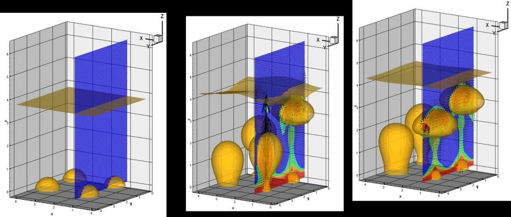
Figure 1. Nucleate Boiling of water at 1atm, Tsat=373.15K; liquid/vapor density ratio=1605; viscosity ratio=23; thermal conductivity ratio=27; specific heat ratio=1; domain size: 10.5x10.5x15.75 mm; Wall superheat: 18K. 40x40x60 grid resolution

Figure 2 : Click here for a movie of the sequence shown in Fig. 1

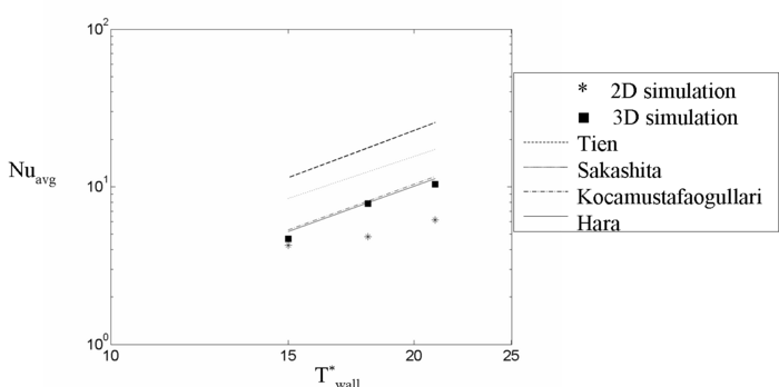
A study of the effect of nucleation site density on heat transfer is shown in Figure 3. This is a plot of wall superheat vs Nusselt number and compares the results for 3D and 2D simulations with several experimental correlations which explicitly take into account nucleation site density. Although the overall level of heat transfer varies among the correlations, they all agree on the trend in Nusselt number with increasing wall superheat. The 3D simulation shows a markedly better agreement in the trend than does the 2D simulation. This suggests that, even under the idealized conditions used in our simulations, the three-dimensional effect of nucleation site density is very important for predicting the proper relationship between heat flux and the wall superheat for a realistic surface.

Figure 3. Comparison of heat transfer results for both 2D and 3D computations vs correlations. (From Shin et al, 2005)

Conclusions

For simulations of nucleate boiling to be meaningful for practical applications it will be necessary to follow the nucleate boiling process from a sufficiently large sample of nucleation sites for a sufficiently long time so that average behaviors can be studied. Obviously the computational cost to achieve sufficient resolution of all of the length scales involved is prohibitive. The main challenge for such simulations is twofold. We must, first of all, be able to capture the microscale physics of the contact line and evaporation near the contact line as the vapor bubbles grow. We are approaching this challenge through an effort on two fronts: (1) increased computational efficiency through parallelization (ongoing joint work with J. Chergui of LIMSI) and (2) subgrid scale modeling. Some progress has already been made in modeling of the microlayer although the physics in this region is still poorly understood and we are evaluating several models. An important aspect of the modeling in this microregion must involve temperature variation in the solid wall which we have not yet treated. Another challenge is the modeling of a realistic nucleation site distribution and the physical characteristics of a real surface. Although a topic of considerable experimental studies, this issue remains mostly unexplored in the context of Direct Numerical Simulations of boiling. The first step is to understand the effect of the site density distribution in general, using artificially generated distributions. Relating such results with real surfaces remains a subject of future study.

References

J.M. Delhaye. Jump Conditions and Entropy Sources in Two-Phase Systems. Local Instant Formulation. Int. J. Multiphase Flow, 1, 395 (1974).

D. Juric and G. Tryggvason, Computations of Boiling Flows, Int. J. Multiphase Flow , 24(3) 387-410 (1998).

C.S. Peskin, Numerical Analysis of Blood Flow in the Heart, J. Comp. Phys. 25, 220-252 (1977).

S. Shin and D. Juric, Modeling Three-Dimensional Multiphase Flow using a Level Contour Reconstruction Method for Front Tracking without Connectivity, J. Comp. Phys., 180, 427-470 (2002).

S. Shin, S.I. Abdel-Khalik, D. Juric, Direct Three-Dimensional Numerical Simulation of Nucleate Boiling using the Level Contour Reconstruction Method, Int. J. Multiphase Flow, 31, 1231-1242 (2005).

S. Shin and D. Juric, High order Level Contour Reconstruction Method, J. Mechanical Science and Technology, 21(2), 311-326 (2007a).

S. Shin and D. Juric, Numerical Simulation of Multiphase Flow using the Level Contour Reconstruction Method : Part II. Contact Line modeling, J. Comp. Phys. (submitted sept. 14, 2007b).

G. Son, V.K. Dhir, and N. Ramanujapu, Dynamics and Heat Transfer Associated With a Single Bubble During Nucleate Boiling on a Horizontal Surface. J. Heat Trans. 121, 623-631 (1999)

P.D.M. Spelt. A level-set approach for simulations of flows with multiple moving contact lines with hysteresis. J. Comp. Phys. 207, 389-404 (2005).

S. O. Unverdi and G. Tryggvason, A Front-Tracking Method for Viscous, Incompressible, Multi-Fluid Flows, J. Comp. Phys. 100, 25-37 (1992).

P.C. Wayner, Jr. Evaporation and Stress in the Contact Line Region. Proc. Eng. Foundation Conf. on Pool and External Flow Boiling. V.K. Dhir and A.E. Bergles, eds. Santa Barbara, CA, 251-256 (1992).

Hara, T. The mechanism of nucleate boiling heat transfer. Int. J. Heat Mass Transfer, 6, 959-969 (1963).

Kocamustafaogullari, G. and Ishii, M. Interfacial area and nucleation site density in boiling systems. Int. J. Heat Mass Transfer, 26, 1377-1387 (1983).

Sakashita, H. and Kumada, T. Method for predicting boiling curves of saturated nucleate boiling. Int. J. Heat Mass Transfer, 44, 673-682 (2000).

Tien, C. L. A hydrodynamic model for nucleate pool boiling. Int. J. Heat Mass Transfer, 5, 533-540 (1962).

Links

Home > Group Solid-Fluid Transfers >> This page