TSF: liquid-gas flows
Contents |
Numerical simulations of liquid-gas flows in enclosures
I. Elayyadi, V. Daru & M.-C. Duluc P. Le Quéré
Objectives
Twophase flows abound in industrial or natural configurations, and their accurate prediction is thus of great interest. For optimization purposes, macroscopic models which do not consider the detailed dynamics of each phase are needed. These models rely on modelling assumptions of the various and complex interactions between each phase. Modelling these interactions require a detailed examination of the phase interactions, and numerical simulations represent a challenging alternative to classical experimental investigations, due to the difficulty of accessing experimentally to all the physical quantities needed for such investigations. In the context of numerical simulation of multiphase phenomena with phase change, the direct numerical simulation (DNS) of liquid vapour flows at microscopic scale is an interesting subject. Indeed, this method allows understanding and ameliorating the closing models used in industrial multiphase codes.
Most previous numerical simulation of flows with bubbles (with or without phase change) assume that the Mach number is very low, and consider that both phases are incompressible. The model is then incompressible multiphase Navier-Stokes system.
Our objective is to obtain a code dealing with:
• Important heat exchange between two phases.
• The fact that at least one of the two phases is strongly compressible (vapour )
• Existence of phase change phenomena water-vapour/ water-vapour
These objectives exclude in our context the incompressible multiphase Navier-Stokes system in favour of the compressible multiphase Navier-Stokes system, although the Mach number is very low.
However, this numerical discretization of compressible system with low Mach number, can be difficult because of the important difference between sound and flow velocity. We propose then to simplify the Compressible system with asymptotic development in power of puissance of Mach number. A low Mach number approximation is used for the vapour allowing for the filtering of the acoustic wave.
Description
The model is based on a single field-formulation. Both phases are described using one single set of equations, i.e. compressible Navier-Stokes equations using the Low Mach number approximation. In this approach developed by Chenoweth and Paolucci (1986), the pressure is split in two components, one is the thermodynamic pressure  solely function of time and the other is the dynamic pressure function of both time and space
  .
.
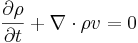
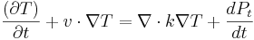
the resulting Navier-Stokes equations are:


The fluid density : 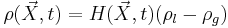 . The liquid is incompressible of density
  .
The assumption of an ideal gas is made for the vapour phase whose density thus reads:
.
The assumption of an ideal gas is made for the vapour phase whose density thus reads:  .
.
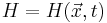 is the Heaviside function used to distinguish the liquid (H=0) from the vapour (H=1)
phase. Its evolution, governed by an advection equation, is solved on a fixed grid using a fronttracking
method as proposed by Tryggvason et al (2001).
The other physical properties required in equation (1) are computed using the generic relation:
is the Heaviside function used to distinguish the liquid (H=0) from the vapour (H=1)
phase. Its evolution, governed by an advection equation, is solved on a fixed grid using a fronttracking
method as proposed by Tryggvason et al (2001).
The other physical properties required in equation (1) are computed using the generic relation:  with :
Numerical Procedure
Given the proper initial boundary conditions, the mathematical formulation presented in the former section is solved as follows:
Spatial resolution is performed using a second-order central finite scheme. Time discretization uses a first second order backward Adams scheme. The computation of the various quantities from time  to
to  is carried out with the following procedure :
Algorithm
-


 and
and 
Results
Conclusions
References
[1] Paolucci S. (1982). On filtering of sound from the Navier-Stokes equations. Sandia National lab. Report SAND, 82-8257, non publié.
[2] D.Juric, V.Daru, M-C.Duluc. (2004). Simulation d'écoulements liquide-gaz à l'intérieurd'une cavité chaufée, SFT Prsqu'ile de Giens.
[3] S.Shin, S.I.Abdel-khalil, V.Daru, D.Juric. (2005). Accurate representation of surface tension using the level contour reconstruction method. J. Comput. Phys 203, 493-516.
[4] S.Shin, D.Juric. (2002). Modeling three-dimensional multiphase flow uing a level co,tour reconstruction method for front tracking without connectivity. J. Comput. Phys 180, 427-470.
[5]