Low order dynamical systems for the generation of unsteady boundary conditions in the LES framework
F. Abéguilé, L. Lorang-Vo Dinh, C. Perrotin, Y. Fraigneau, B. Podvin, L. Mathelin, O. Le Maître and C. Tenaud
Contents |
Object
The aim of this work is to derive a reduced, comprising a limited number of degrees of freedom, representation of an initially complex system. In many situations, the system to model or simulate is far too complex to be handled by current computers and numerical algorithms in a reasonable amount of time. This intractability may come from coupled physical phenomena or a very large space- or time-scale ratii within the system. In the present context of numerical fluid mechanics, rather than dealing with a huge number, say billions, of mesh cells, the approach developed here is that of deriving a compact, low dimensional, manifold onto which the original system may be projected. The manifold is chosen so as the dynamics of the projection is sufficiently close to the original one. In addition to its accuracy in terms of dynamics, the reduced system also has to be able to handle various operating conditions or parameters set for the system. More specifically, a reduced model derived for, say, a certain Rayleigh number has to remain accurate for a different Rayleigh number flow realization and the reduced model is then termed robust.
In our department, we develop different reduced model strategies that have been tested on several cases, we have chosen to detail some of them: (1) the derivation of a reduced robust basis for the 2-D flow around a circular cylinder using a mapping method, (2) the modeling of wall-layer boundary conditions on moderate Reynolds incompressible channel flows with POD Galerkin projection and neural identification (3a) the generation of inlet conditions of compressible channel flows and (3b) the reduction of a mixing layer flow using neural network tools.
Flow around a circular cylinder
The considered configuration is that of a circular cylinder in cross-flow. Due to its time-consuming character and to the perspective of real-time flow control, it is necessary to derive a much "lighter" model. In addition to that, the flow Reynolds number  may be poorly known as this is representative of the configuration of an airplane wing in actual flight where the incident fluid velocity may vary. Further, the control of the flow is applied by sucking or blowing some fluid through the cylinder surface with a prescribed intensity
  .
.
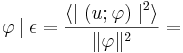
The reduced basis thus has to be robust against both the Reynolds number and the control intensity. In the POD method one looks for a basis spanned by vectors  satisfying
 ,
, ![\varphi \in \mathcal{L}^2([0;1])](../upload/math/d/b/a/dba457e12af68a3b81a0fb18f371e831.png)
which is further subjected to  with
with 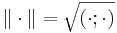 the
the  -norm. A problem variable
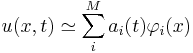
  can then be approximated as
The bracket product  denotes the ensemble average operator and
  a scalar product.
After little algebra, we finally end up with a Fredholm equation :
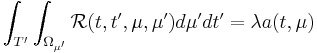
with  the probability density function. This defines an eigenvalue problem.
  is the autocorrelation matrix. The eigenvectors
  form an orthogonal set satisfying
with  the Kronecker symbol. This formulation thus intrinsically integrates the statistical character of and through the
  and
and  terms.
We define the mapping  which updates the POD coefficients
  over the time-horizon
  :
:
The time integration of the system is thus simply the successive application of the mapping over the time horizon and is done at extremely low CPU cost.
Results and prospects
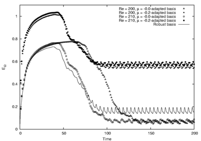
Figure 1 shows the error representation of the flow field at  by different reduced basis. After the transient phase, the base derived from -snapshots exhibits a very low error while the performance is much worse when one uses a basis derived from a
  -snapshots series. While achieving a lower performance, the robust basis still gives a reasonable approximation of the flow. Applying the same criterion to a -flow field, conclusions are the same: the basis achieves a very good performance while the one derived from a -flow field does a very poor job and the robust basis still provides an acceptable approximation. One can thus conclude that while never achieving the best performance for a specific Reynolds number, the robust basis remains relevant on a whole range of operating parameters (Reynolds number here).
 |
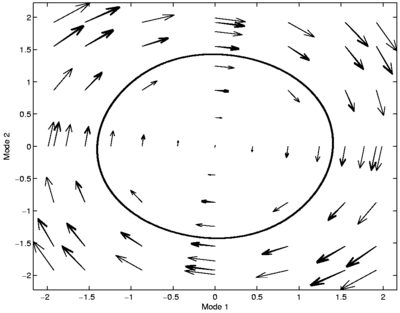 |
Figure 2 presents the mapping in the  -
-  -plane. The limit cycle obtained by DNS is also plotted and is accurately approached as the POD coefficients are time-integrated using the mapping scheme, proving the validity of this approach.
Boundary layer modeling
The Galerkin projection
Dynamical systems for the full flow can be obtained by projecting the Navier-Stokes equation onto the full 3-D POD representation basis.
POD-based, low-order dynamical systems (LODS) have been derived for the wall layer of a turbulent channel flow at different Reynolds numbers.
This is part of the project WALLTURB, which aims at a better, global characterization of wall turbulence by combining experimental results,
numerical simulations and turbulence modeling. One of the objectives of WALLTURB is LES/LODS coupling: low-order models could be used to represent the flow in the lower part of the wall layer, which remains inaccessible to large-eddy simulations. We have used numerical data
from UPM Madrid, as well as our own DNS code at LIMSI to carry out the 3-D POD analysis and build the corresponding models. We find that the first POD eigenfunctions
and eigenvalues are essentially the same for  between 100 and 1000. A comparison between the full numerical simulation
and the LODS prediction shows that exact correspondence is difficult to establish, but that some intermittent features of the bursting process are adequately captured.
The coupling procedure is currently being implemented.
between 100 and 1000. A comparison between the full numerical simulation
and the LODS prediction shows that exact correspondence is difficult to establish, but that some intermittent features of the bursting process are adequately captured.
The coupling procedure is currently being implemented.
Neural identification
Classically, dynamical systems are obtained via a projection of the Navier-Stokes equations on the POD base (POD-Galerkin). The main drawback of Galerkin projection method, is that the boundary conditions are to be known precisely and that the velocity field has to be known at a sufficient resolution to prevent from numerical noise as the spatial POD modes derivatives intervene. The influence of the neglected modes (dissipation) as the pressure contribution are to be modeled.
The problem is the following, we have to determine  functions
  , where is the number of modes, so that:
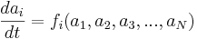
By integrating this relation, we obtain the dynamic behavior of the system. The integration of the function  is carried out by an integration of Runge-Kutta type (
 order), from an initial condition given by the original temporal coefficients. The problem can be treated differently by including the integration process in the function identification, we have then:

The neural network consists in finding the weights  so that:
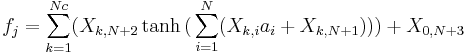
 is the number of hidden units. This type of equation is called multilayer perceptron and is very efficient in the framework of nonlinear regression. During the training a simplex algorithm is used to minimize the error between the estimated function and the samples. Among universal approximators, neural networks exhibit a remarkable property, namely parsimony: the number of adjustable parameters required to approximate a given function with a given precision is much smaller than the number of parameters required for conventional approximators (polynomials, Fourier series, etc.). The robustness of a network does not rest only on its ability to reproduce the sequence on which the learning was performed, but also on its ability to reproduce an unknown sequence. In theory, the more a network is complex, i.e. the higher is the number of units in the hidden layer, the more it will be able to reproduce faithfully the learnt sequence. Nevertheless, it can result in a loss of generalization and lead to a worth estimation of other sequences. A compromise must be found between these two types of estimation. The number of coefficients to determine for each mode is
  . So this method is relevant for large number of modes if we keep a low value of Nc.
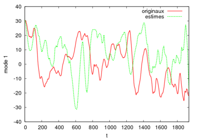
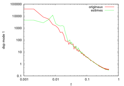
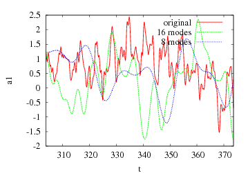
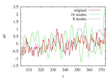
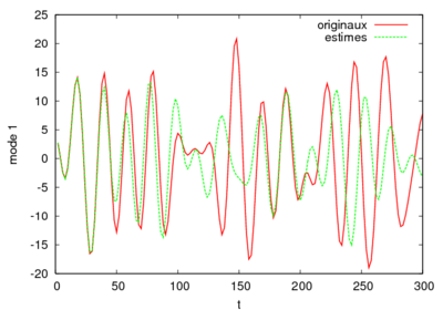
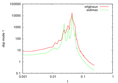
We have applied this methodology on experimental PIV data provided by the LML in the frame of the CALINS-project. The data consist in 1936 consecutive snapshots of a turbulent boundary flow at R_theta=7800. The POD based on the velocity field on a plane located at y+=100 was performed by M. Girault in Poitiers. Surprisingly, our model turns out to be able to reproduce with good agreements the low-frequency dynamics. Moreover our system is stable in time without adding any eddy-viscosity. To get more accuracy in our reconstruction we still have to improve the high-frequency prediction. The evolution of the dynamical system for the first POD mode and his associated spectrum are represented in figure 3 and 4.
 |
 |
Inlet conditions modelling
The objective of this work is to set up an inflow condition generator for simulations of fully developed turbulent flows. First we extracted the dominant structures of the flow thanks to three kind of POD approaches. Then we injected the reconstructed fluctuations at the inlet in order to minimize the characteristic length from which an equilibrium turbulent boundary layer is recovered. The idea was then to predict the evolution of the temporal coefficients by means of dynamical systems. Even if the configuration studied here is simple, it has nevertheless all the dynamics of a fully turbulent and compressible flow.
Different POD approaches
To generate fluctuating quantities with a space-time distribution characteristic of the turbulent flow, a POD was carried out in an arbitrary section of the channel [5]. The Reynolds number (based on the channel half height and mean velocity) was  , corresponding to
 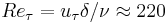 , and the Mach number was 1,5. To improve the representation of the correlations between the various quantities, we considered a POD performed independently on each conservatives variables (scalar POD) and a POD where these last ones are coupled (vectorial POD). To reduce the dimension of the considered systems, this procedure was performed in the spectral space. In the homogeneous directions of the flow, the POD is reduced to a harmonic decomposition [1], one thus applies beforehand a Fourier decomposition to the fluctuations of the conservative variables
 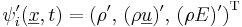 in the transverse direction. In the POD base, the fluctuating field is estimated as follows :
 ,
where
,
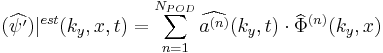
where  is the number of modes retained for the reconstruction. Temporal coefficients associated to POD modes are given by :
 where
where  is the eigenfunction associated to the
  eigenvalue
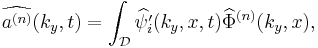
  of the two-point space correlation tensor
  .
Considering then a channel in spatially developing flow, of finite length, with specific boundary conditions at the inflow (mean field + reconstructed fluctuations) and at the exit (condition of not reflexion) handled by the method of characteristics, the objective is to reproduce the precursor simulation (with periodic streamwise boundary conditions). The advantage of the spectral approach lies essentially in the compression of the volume of data connected to the construction of generators.
.
Considering then a channel in spatially developing flow, of finite length, with specific boundary conditions at the inflow (mean field + reconstructed fluctuations) and at the exit (condition of not reflexion) handled by the method of characteristics, the objective is to reproduce the precursor simulation (with periodic streamwise boundary conditions). The advantage of the spectral approach lies essentially in the compression of the volume of data connected to the construction of generators.
|
Kind of POD |
POD scalaire |
POD pseudo-vectoriel |
POD vectoriel |
|---|---|---|---|
|
Size of the problem |
|
|
|
|
Modes for 0.999 |
|
|
|
|
Error |
|
|
|


Table 1. For the three spectral approaches: size of the autocorrelation matrix, number of modes selected and error (L1-morm) committed on the real field for 99,9% of the energy
Neural identification
The training is realized on the temporal coefficients which are this time complex numbers. We proceed as described in (ref), the imaginary part and real part has been treated separately.
 |
 |
Spatially developped mixing-layer flow
The aim of this work was to model the temporal evolution of the  coefficients starting from given samples of and
  . Three different methods have been compared in this particular case : the Galerkin projection, polynomials identification and neural network identification which were respectively addressed by TU-Berlin, LEA-Poitiers and LIMSI. The initial flow was computed with LES by Comte at IMFS-Strasbourg.
All the different  have been integrated trough a fourth order Runge-Kutta Method, the result obtain can be seen on fig.7 and fig.8. All the methods show good reliability in short-term calculation. The long-term performance is fairly awkward as a phase shift appear rapidly after 4 or 5 time-period. As real-time control only need mean-term calculation, this kind of reduced system can be used as a part of a closed loop system: the predicator, which parameters are to be updated by wall measurements.
 |
 |
Conclusion
Much efforts have been dedicated to reduced order modelling in our department. Our purpose now is to compare the different strategies we have implemented to see their pros and cons on similar cases. Neural networks are very seducing tools as we have proove their capability of reproducing complex flows at small cost but their is still some development to do on the minimization procedure. Galerkin projection is closer to the physics and is still the reference in the Low Order Modelling community. The main effort has to be put on a better modelisation of the dissipation coefficient.
References
[1] Lumley J.L., The structure of Inhomogeneous Turbulent Flows, In Atmospheric turbulence and radio propagation, edited by A.M. Yaglom and V.I. Tatarski, Moscow: Nauka, p. 166-178, 1967.
[2] Holmes P., Lumley J.L. & Berkooz G., Turbulence, coherent structures, dynamical systems and symmetry, Cambridge University Press, 420 p. 1996.
[3] Perret L., Etude du couplage instationnaire calculs-expériences en écoulements turbulents, PhD thesis, Laboratoire d'Etudes Aérodynamique, Poitiers, France, 2004.
[4] Dreyfus G. collectif, Réseaux de neurones, édition Eyrolles, 417 p. 2004.
[5] Abéguilé F., Fraigneau Y., Lorang L. & Tenaud C., Générateur de conditions aux limites amont pour les simulations de type LES des écoulements de paroi. XVIIIème Congrès Français de Mécanique, Grenoble.
[6] Bergmann M., Optimisation aérodynamique par réduction de modèle POD et contrôle optimal. Application au sillage lamainaire d'un cylindre circulaire, Thèse de Doctorat, Institut National Polytechnique de Lorraine. France, Nancy.