Adaptive Mesh Refinement for unsteady shocked flow simulations
Contents |
Object
In the high speed flow regime, many aerodynamic configurations involve interactions between shock waves and flow inhomogeneities such as, for instance, within air intake configurations where shock wave/turbulent shear layer (e.g. boundary layer) interactions occur. At the present time, it is commonly admitted that advanced numerical simulations (DNS or LES) are powerful tools for accurate predictions of shock wave turbulent shear layer interactions including large-scale flow phenomena. Following the LES approach, the quality of the solutions not only depends on the capability of the numerical scheme associated with sub-grid modellings but also depends on the ability of the computational grid to capture the governing dynamical process. In fact, some phenomena could not be accounted by sub-grid modellings and accurate schemes coupled with locally very fine adapted grid are needed to recover a high quality of the solution. For instance, according to the theoretical developments in the Linearised Interaction Approximation, the shock-wave/turbulence interaction phenomenon requires the correct prediction of the shock wave deformation occurring at small scales. These small scale shock deformations which could not be accounted by LES modelling, need locally very fine grid. The production of vorticity through baroclinic effect is also a phenomena largely encountered in real flow physics that could not be accounted by sub-grid modellings and needs accurate numerical scheme on grid tightened in the production regions. These examples show that it is necessary to dynamically refine the grid locally, in the regions where the unsteady phenomena occur. It then motivates the introduction of self-adaptive discretization, as the solution may be over-resolved in large subsets of the computational domain when using equidistant fine grids. Therefore, to be efficient in terms of CPU time and memory usage, Adaptive Mesh Refinement (AMR) must be employed to save grid points in smooth regions and to concentrate them in the regions where phenomena (discontinuity, vorticity production, ...) occur. To be adequate for the DNS or LES approaches, the AMR techniques must be based on Multi-Resolution Analysis (MRA) to offer a reliable error control of the solution. This study aims at contributing to the assessment of the finite volume multi-resolution analysis to recover the basic interactions in fluid mechanics. The main objective is to evaluate the capability of the a dynamical adaptive mesh refinement algorithms, based on error estimates coupled with high-order shock capturing schemes, to capture small scale mechanisms, encountered in many aerodynamic flows, that have no concern with classical sub-grid scale models. This evaluation is performed on numerical simulations of basic 2D compressible flows: the Euler advection of a vortex, the shock-wave / spot of temperature viscous interaction, the shock-wave / vortex interaction and the viscous shock tube.
Description
Adaptive discretizations for problems exhibiting locally stiff gradients or shock-like structures have been used since the end of the 1970s. Historically, adaptive methods like Multi-Level Adaptive Techniques (MLAT) [Brandt (1977)] or Adaptive Mesh Refinement (AMR) [Berger et al. (1984, 1989)] were the first to achieve this goal, using a set of locally refined grids where stiff gradients of high truncation errors are found. However, the data compression rate is high where the solution is almost constant, but remains low where the solution is regular. To overcome this difficulty, adaptive multiresolution methods, based on Harten's pioneering work [Harten (1995], have been developed for 1D and 2D hyperbolic conservation laws [Gottschlich-Müller et al. (1999), Cohen et al. (2003)]. They have then been extended to 3D parabolic problems [Roussel (2003)]. It has been shown in these papers that a high compression rate can be reached for solutions with inhomogeneous regularity. For an overview on adaptive multiresolution techniques, you can refer to the books of Cohen (2000) and Müller (2003).
The principle of the multiresolution analysis is to represent the data on a set of nested dyadic grids. The data given on a fine grid is decomposed into values on a coarser grid plus a series of differences at different levels of dyadic grids. These differences contain the information of the solution when going from a coarse to a finer grid. In particular, these coefficients are small in regions where the solution is smooth and yield hence high compression rates for functions with inhomogeneous regularity. A tree structure is used to code the solution. The tree structure is composed of a root cell, which is the basis of the
tree, the nodes which are elements of the tree, and the leaves which are the upper elements. In  dimensions, a parent cell at a level
  has always
  children cells at the level
  . Each node of the tree contains the cell-average value of the solution. To compute the average value of a cell at level from the cell values at a finer level , we use the projection (or restriction) operator
  . It is exact and unique, given that the cell-average value of a parent cell is the weighted average value of its children cell-averages. The prediction (or prolongation) operator
  maps the solution at level to an approximation of the solution at level . In contrast with the projection operator, there is an infinite number of choices for the definition of . Nevertheless, in order to be applicable in a graded tree structure, it needs to be consistent with the projection, i.e.
  , and local, i.e. based on an interpolation using the
  nearest neighbours in each direction. The detail is the difference between the exact solution on level and the predicted value. Thanks to the consistency assumption, the sum of the details on all the children of a parent cell is equal to zero. Therefore, in dimensions, the knowledge of the children cell-averages of a given parent cell is equivalent to the knowledge of the parent cell-average and
  details. Repeating this operation on all the $L$ levels, one gets the so-called multiresolution transform [Harten (1995)] . The threshold operator consists in removing leaves where details are smaller than a prescribed tolerance
  , without violating the graded tree data structure. The tolerance is chosen such that the discretization error of the reference numerical scheme is balanced with the accumulated threshold error. To ensure a strict conservativity in the flux computation between cells of different levels, without increasing significantly the number of costly flux evaluations, we compute only the fluxes at the level and set the ingoing flux on the leaf of level equal to the sum of the outgoing fluxes on the leaves of level .
The space and time discretizations are performed through a Lax-Wendroff approach by using the high-order shock capturing scheme (OSMP7) [Daru et al. (2004)] developed at LIMSI.
, without violating the graded tree data structure. The tolerance is chosen such that the discretization error of the reference numerical scheme is balanced with the accumulated threshold error. To ensure a strict conservativity in the flux computation between cells of different levels, without increasing significantly the number of costly flux evaluations, we compute only the fluxes at the level and set the ingoing flux on the leaf of level equal to the sum of the outgoing fluxes on the leaves of level .
The space and time discretizations are performed through a Lax-Wendroff approach by using the high-order shock capturing scheme (OSMP7) [Daru et al. (2004)] developed at LIMSI.
Results and prospect
The capability of the present approach is checked on test-cases chosen here to deal with interactions between wave propagations and shock phenomena. It is a first step to recover very elementary phenomena that contribute to the turbulence production. The aim here is to perform computations in several configurations and to assess the efficiency and the accuracy of the adaptive multiresolution (MR) method coupled with a high-order shock-capturing scheme. The classical finite volume scheme on the regular finest grid is denoted by (FV) while the adaptive multiresolution scheme is denoted by (MR). A parametric study on the tolerance to find the largest value for which the discretization error of the numerical scheme is balanced with the accumulated threshold error. Errors are computed in  -norm. The performance analyses enable us to show if the choice of a MR algorithm is justified for such computations.
Several classical 2D inviscid (advection of a vortex) or viscous test-cases (shock/hot spot or shock/vortex interactions and shock tube problem) have been computed to validate the present approach.
-norm. The performance analyses enable us to show if the choice of a MR algorithm is justified for such computations.
Several classical 2D inviscid (advection of a vortex) or viscous test-cases (shock/hot spot or shock/vortex interactions and shock tube problem) have been computed to validate the present approach.
Convergence study for a 2D Euler case:
We consider the propagation at  to the grid lines of a strong vortex at a supersonic Mach number. This test-case is the one studied in [Balsara et al. (2000) and Daru et al. (2004)]. The vortex is initially centred in the computational domain. Periodic boundary conditions are imposed. The exact solution is just the passive convection of the vortex. This test-case must highlight the accuracy of the present method and its capability to recover vorticity conservation. The errors are calculated at time
  .
.
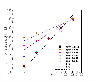 Figure 1: Advection of a vortex: errors versus the mesh size ( ), influence of the threshold level () of the MRA method. ), influence of the threshold level () of the MRA method. |
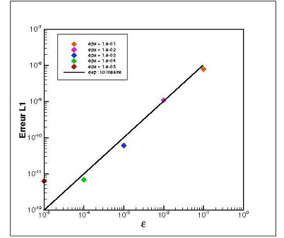 Figure 2: Advection of a vortex: errors scale linearly versus the threshold level () of the MRA method. |
In Figure 1 are plotted the errors obtained using the OS7 scheme. We can see that this scheme is only fifth order accurate, due to the simplified extension to the non linear system case. Nevertheless, magnitudes of errors are indeed much lower than for a classical uncoupled time-space scheme of the same order [Balsara et al. (2000)]. When the threshold is less than  , the accuracy is not altered by the Multi-Resolution (MR) algorithm. For greater values, the thresholding error dominates the global error of the solution.
 .
.Figure 2 is dedicated to the evaluation of the perturbation error, i.e. the error of the MR algorithm compared to the Finite Volume (FV) solution, due to the accumulated MR thresholding error. In other words, this error increases with the tolerance , whereas the CPU time decreases when increases. Compared to the FV approach using a single grid, we demonstrated that CPU time can be saved by the MR approach when more than 50 % of the mesh cells are dilated from the memory. This is reached when the highest-level mesh is sufficiently fine and the threshold () is rather high, i.e.  . On Figure 2 we can also notice that the threshold perturbation error has a linear fit versus the threshold parameter which is in complete agreement with the heuristic MR approach from Harten's work [Harten (1995)]. At time
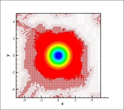
  , the vortex is return to its initial place. Then, we can see on Figure 3 the adapted mesh concentrated around the region where gradients occur.
2D viscous interaction between a weak shock-wave and a spot of temperature:
The goal of this test-case is to investigate the capability of the present method to predict the vorticity production induced by baroclinic effects. Recall that only baroclinic effects are capable of producing vorticity in 2D inviscid flows. This test-case is the one studied in [Tenaud et al. (2000)]. A hot-spot of temperature is initially superimposed (as an isobaric perturbation of temperature) to a uniform flow at a reference Mach number  and a Reynolds number
  , in front of a steady plane weak shock-wave. To compare with, the reference solution is obtained by means of the sixth-order accurate Hermitian scheme [Tenaud et al. (2000)]. The time histories of the integral of the magnitude of the vorticity and the magnitude of the baroclinic torque are plotted in Figures 4 and 5. On these figures, the present approach is compared to the reference. At the initial time (
 ), the vorticity and the baroclinic torque are zero. At a dimensionless time
  , the temperature spot starts to interact with the shock wave. The maximum of the production of vorticity occurs at about
  when the centre of the temperature spot coincides with the shock location. The present method agrees very well with the reference thanks to the MR approach coupled with the high-order shock capturing scheme (OSMP7) (Figure 4 and 5).
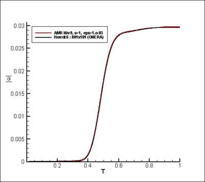 ) and compared to the reference solution (6th-order Hermit scheme on single fine grid). ) and compared to the reference solution (6th-order Hermit scheme on single fine grid). |
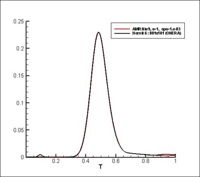 ) and compared to the reference solution (6th-order Hermit scheme on single fine grid. ) and compared to the reference solution (6th-order Hermit scheme on single fine grid. |
At , the iso-values of the density (Figure 6) show a modification in the curvature of the shock. The vorticity is produced within and just downstream the shock (Figure 6); the final product being a pair of counter-rotating vortices. Since the initial temperature distribution is symmetric, the vorticity field is anti-symmetric with respect to the centreline of the domain. As the spot is convected downstream of the weak shock, the intensity of the baroclinic torque decreases rapidly (Figure 5). At  , the temperature spot still interacts with the shock as shown in (Figure 7) as the shock is still bent. The production of vorticity keeps a residual value at the final time of the computation (Figure 5). The vorticity is concentrated in two counter-rotating vortices and no vorticity is present within the shock (Figure 7). The corresponding meshes at time
  are also shown on Figure 6 and 7. We can notice that the grids are embedded over 6 levels (from 4 to 9) and the higher levels (finer meshes) are concentrated in the region where gradients occur. Using this value of the threshold, the memory compression rates are about 46 % and 61 % respectively at dimensionless times (Figure 6, bottom) and (Figure 7, bottom). These compression rates lead to CPU times equivalent to the ones of the FV approach on a single grid. For greater values, gains in CPU time and memory usage are much larger and the present method remains competitive compared to FV approach with equivalent accuracies.
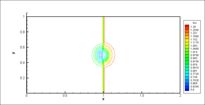 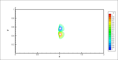 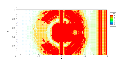 Figure 6: Interaction between a spot of temperature with a weak shock-wave at |
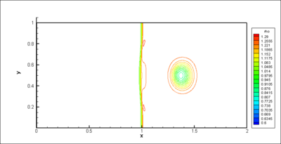 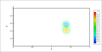 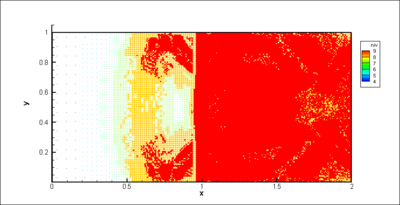 Figure 7: Interaction between a spot of temperature with a weak shock-wave at |
Movies on the solution from 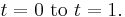 ]] can also be seen on [the density countours], [the vorticity countours] and
[the corresponding adapted grid], using 9 grid levels (finest grid: 1024x512) and .
]] can also be seen on [the density countours], [the vorticity countours] and
[the corresponding adapted grid], using 9 grid levels (finest grid: 1024x512) and .
2D viscous interaction between a weak shock-wave and a vortex:
This test-case has been chosen to highlight the capability of the present MR method to predict the generation and the transport of acoustic waves during a shock-vortex interaction. The study is restricted to the interaction of a plane weak shock with a single isentropic vortex. The intensity of the vortex is weak enough to deal with low shock deformations during the interaction so that the linear theory can be applied. This test-case is similar to the one studied in [Tenaud et al. (2000)]. An isentropic vortex is prescribed in front of a steady plane weak shock-wave. The Mach number of the base flow at infinity is and the Reynolds number is . The final dimensionless time of the computations is 0.7. At the beginning of the shock-vortex interaction (), a circular acoustic wave propagating at the speed of sound is generated. This wave is clearly seen in Figure 8, where the static pressure is plotted. These presented results have been obtained by using the OSMP7 scheme coupled with the present MR method using 9 grids levels and a threshold . The vortex, located just behind the shock, has an elliptic shape whose main axis is parallel to the shock, in agreement with the prediction of the Rapid Distorsion Theory. The adapted grid is dynamically tightened in regions where gradients occur. We must notice that the dynamical grid adaptation clearly follows the acoustic waves produced (see movies hereafter). For this value, the memory compression rate is about 50 % at  compared to the single grid of the FV approach, leading to a slightly smaller CPU time than the one used in the FV approach. For greater values, gains in CPU time and memory usage are much larger and the present method remains competitive compared to FV approach with equivalent accuracies.
 : iso-contours of the static pressure (25 contours from 0.527 to 0.845), computed by using the MRA method coupled with the OSMP7 scheme (9 grid levels, 512x512, ). : iso-contours of the static pressure (25 contours from 0.527 to 0.845), computed by using the MRA method coupled with the OSMP7 scheme (9 grid levels, 512x512, ). |
 : adapted mesh computed by using the MRA method coupled with the OSMP7 scheme (9 grid levels, 512x512, ). : adapted mesh computed by using the MRA method coupled with the OSMP7 scheme (9 grid levels, 512x512, ). |
Movies on the solution from ]] can also be seen on [the static pressure countours] and
[the corresponding adapted grid], using 9 grid levels (finest grid: 512x512) and .
2D viscous shock tube problem:
We consider a unit side length square shock tube with insulated walls. The diaphragm is initially located in the middle of the tube. The initial state is the one of the test-case studied in [Daru et al. (2001)]: the flow is at rest with a high pressure on the left-side of the diaphragm and a low-pressure on the right-side. At the initial time, the diaphragm is broken. A shock wave, followed by a contact discontinuity, moves to the low-pressure region (i.e. to the right, for instance), while rarefaction waves move to the high-pressure region (i.e. to the left, for instance). The incident shock wave reflects at the right end wall
approximately at time  . After this reflection, it interacts with the contact discontinuity. Complex interactions then occur leading to transmitted and reflected waves. Afterwards, the contact discontinuity stays stationary, close to the right end wall. The reflected shock wave moves on and begins to interact with the rarefaction wave at time
  . These rarefaction waves reflect on the left end wall at a dimensionless time , modifying the propagation of the incident rarefaction wave. In the viscous case, the propagating incident shock wave and contact discontinuity interact with the horizontal wall, creating then a thin boundary layer. After its reflection on the right end wall, the reflected shock wave interacts with this boundary layer. As the stagnation pressure in the boundary layer is lower than the one within the outflow region, a dead-water region (named bubble) takes place over a large extent within the boundary layer, resulting in a major modification of the flow pattern and the formation of
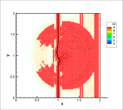
a lambda-shape like shock pattern. The triple point emerging from the lambda-shape like shock pattern generates a slip line that rolls up around the vortex situated at the bottom of the contact discontinuity (bottom right corner). The MRA solution obtained at (Figure 10) on an adapted grid compares very well with the FV solution, using the same scheme (OSMP7). Compared to the FV approach on a single grid, the memory compression rate is 74 % at the final time, allowing a substantial gain in the CPU time. Compressions in memory and CPU time are mainly efficient in the first time of the computation, before waves hit the right-end wall (
. These rarefaction waves reflect on the left end wall at a dimensionless time , modifying the propagation of the incident rarefaction wave. In the viscous case, the propagating incident shock wave and contact discontinuity interact with the horizontal wall, creating then a thin boundary layer. After its reflection on the right end wall, the reflected shock wave interacts with this boundary layer. As the stagnation pressure in the boundary layer is lower than the one within the outflow region, a dead-water region (named bubble) takes place over a large extent within the boundary layer, resulting in a major modification of the flow pattern and the formation of
a lambda-shape like shock pattern. The triple point emerging from the lambda-shape like shock pattern generates a slip line that rolls up around the vortex situated at the bottom of the contact discontinuity (bottom right corner). The MRA solution obtained at (Figure 10) on an adapted grid compares very well with the FV solution, using the same scheme (OSMP7). Compared to the FV approach on a single grid, the memory compression rate is 74 % at the final time, allowing a substantial gain in the CPU time. Compressions in memory and CPU time are mainly efficient in the first time of the computation, before waves hit the right-end wall ( ), because gradients on the conservative quantities are only concentrated close to the wall and in the vicinity of the shock wave and the contact discontinuity.
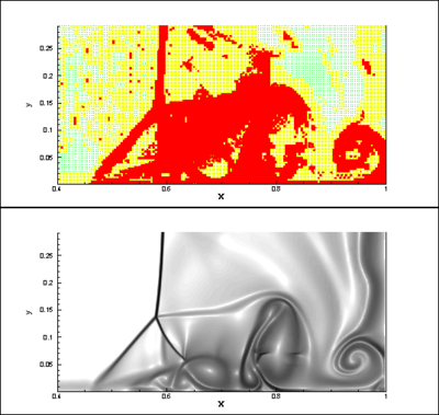 for
for  : numerical schlieren (magnitude of
  gradient, bottom) computed with the MRA method coupled with the OSMP7 scheme by using 9 grid levels (finest grid: 1024x512), ).
At , the time evolution of the solution can be seen [here on the movie] of the iso-contours of the density.
The time evolution of the corresponding adapted mesh can also be seen [here on the movie] (red corresponds to the highest level and blue to lowest level).
Prospect:
The MultiResolution Analysis using wavelet basis is a recent concept that is very attractive compared to more classical AMR approach. We proved on several well documented test-cases that substantial gains in memory usage and CPU time can be achieved when 50 % of the memory is saved compared to a Finite Volume method on a finest single grid. To be more efficient and competitive, the present method needs however further developments:
- the coding of the solution on a tree must be upgraded to allow parallel computing;
- the present algorithm has voluntarily been developed on Cartesian grid to recover the accuracy property of the OSM7 scheme. This leads to develop Immersed Boundary Conditions technique applied to MRA approach to deal with meshes which do not fit the boundaries (especially solid wall).
References
- D. S. Balsara and C.W. Shu (2000), Monotonicity Preserving Weighted Essentially Non-Oscillatory Schemes with Increasingly High Order of Accuracy, J. Comput. Phys., 160: 405-452.
- M. J. Berger and J. Oliger (1984), Adaptive Mesh Refinement for Hyperbolic Partial Differential Equations, J. Comput. Phys., 53: 484-512.
- M. J. Berger and P. Collela (1989), Local Adaptive Mesh Refinement for Shock Hydrodynamics, J. Comput. Phys., 82: 64-84.
- A. Brandt (1977), Multi-level Adaptive Solutions to boundary Value Problems, Math. Comp., 31: 333-390.
- A. Cohen, N. Dyn, S.M. Kaber and M. Postel (2000), Multiresolution Finite Volume Schemes on Triangles, J. Comp. Physics., 161: 264-286.
- A. Cohen, S.M. Kaber, S. M\"uller and M. Postel (2003), Fully Adaptive Multiresolution Finite Volume Schemes for Conservation Laws, Math. Comp., 72(241): 183-225.
- V. Daru and C. Tenaud (2001), Evaluation of TVD High Resolution Schemes for Unsteady Viscous Shocked Flows, Computers and Fluids, 30: 89-113.
- V. Daru and C. Tenaud (2004), High Order One-step Monotonicity-Preserving Schemes for Unsteady Compressible flow Calculations, J. Comput. Phys., 193(2): 563-594.
- B. Gottschlich-Müller and S. Müller (1999), Adaptive Finite Volume Schemes for Conservation Laws Based on Local Multiresolution Techniques. Hyperbolic Problems: Theory, Numerics, Applications, In M. Fey and Jeltsch, eds, pp: 385-394.
- A. Harten (1995), Multiresolution Alogrithms for the Numerical Solution of Hyperbolic Conservation Laws, Comm. Pure Appl. Math., 48:1305-1342.
- S. Müller (2003), Adaptive Multiscale Schemes for Conservation Laws, Habilitation Thesis RWTH Aachen published in Lecture Notes in Computational Science and Engineering, 27, Springer.
- O. Roussel (2003), Développement d'un Algorithme Multirésolution Adaptatif Tridimensionnel pour la Résolution des Equations aux Dérivées Partielles Paraboliques. Application aux Instabilités Thermodiffusives de Flamme, thèse de Doctorat, Université de la Méditerranée.
- C. Tenaud, E. Garnier and P. Sagaut (2000), Evaluation of Some High-Order Shock Capturing Schemes for Direct Numerical Simulation of Unsteady Two-Dimensional Free Flows, Int. J. Numer. Meth. Fluids, 33: 249-278.